AMAZON multi-meters discounts AMAZON oscilloscope discounts
- Transfer Functions, Time Constant and the Forcing Function
- Understanding ‘e’ and Plotting Curves on Log Scales
- Time Domain and Frequency Domain Analysis
- Complex Representation
- Nonrepetitive Stimuli
- The s-plane
- Laplace Transform
- Disturbances and the Role of Feedback
- Transfer Function of the RC Filter
- The Integrator Op-amp (“pole-at-zero” filter)
- Mathematics in the Log Plane
- Transfer Function of the LC Filter
- Summary of Transfer Functions of Passive Filters
- Poles and Zeros
- Interaction of Poles and Zeros
- Closed and Open Loop Gain
- The Voltage Divider
- Pulse Width Modulator Transfer Function (gain)
- Voltage Feedforward
- Power Stage Transfer Function
- Plant Transfer Functions of All the Topologies
- Boost Converter
- Feedback Stage Transfer Functions
- Closing the Loop
- Criteria for Loop Stability
- Plotting the Open-loop Gain and Phase with an Integrator
- Canceling the Double Pole of the LC Filter
- The ESR Zero
- Designing a Type 3 Op-amp Compensation Network
- Optimizing the Feedback Loop
- Input Ripple Rejection
- Load Transients
- Type 1 and Type 2 Compensations
- Transconductance Op-amp Compensation
- Simpler Transconductance Op-amp Compensation
- Compensating with Current Mode Control
Transfer Functions, Time Constant and the Forcing Function
In Section 1 we had discussed a simple series resistor-capacitor (RC) charging circuit. What we were effectively doing there was that by closing the switch we were applying a step voltage (stimulus) to the RC network. And we studied its "response" - which we defined as the voltage appearing across the terminals of the capacitor.
Circuits like these can be looked upon as a "black box", with two terminals coming in (the input, or the excitation) and two leaving (the output, or the response). One of the rails may of course be common to both the input and output, as in the case of the ground rail.
This forms a "two-port network". Such an approach is useful, because power supplies too, can be thought of in much the same way - with two terminals coming in and two leaving, exposed to various disturbances/stimuli/excitations.
But let us examine the original RC-network in more detail first, to clarify the approach further. Let us say that the input to this RC network is a voltage step of height 'vi'.
The output of this network is taken to be the voltage across the capacitor, which we now call 'vo' here. Note that vo is a function of time. We define the ratio of the output to the input of any such two-port network, i.e. vo/vi in this case, as the 'transfer function'. Knowing how the RC network behaves, we also know the transfer function of this two-port network, which is:
vo(t) / vi = 1 - e^-t/RC
Note that in general, a transfer function need not be "Volts/Volts" (dimensionless). In fact, neither the input nor the output of a two-port network need necessarily be voltage, or even similar quantities. For example, a two-port network can be as simple as a current sense resistor. Its input is the current flowing into it, and its output is the sensed voltage across it.
So, its transfer function has the units of voltage divided by current, that is, resistance. Later, when we analyze a power supply in more detail, we will see that its pulse width modulator ("PWM") section for example, has an input that is called the 'control voltage', but its output is the dimensionless quantity - duty cycle (of the converter). So the transfer function in this case has the units of Volts-1.
Returning to the RC network, we can ask - how did we actually arrive at the transfer function stated above? For that, we first use Kirchhoff's voltage law to generate the following differential equation:
....where i(t) is the charging current, q(t) is the charge on the capacitor, vres(t) is the voltage across the resistor, and vcap(t) is the voltage across the capacitor (i.e. vo(t), the output).
Further, since charge is related to current by dq(t)/dt = i(t), we can write the preceding equation as ...
At this point we actually "cheat" a little. Knowing the properties of the exponential function y(x) = ex, we do some educated reverse-guessing. And that is how we get the following solution:
Substituting q = C × vcap, we then arrive at the required transfer function of the RC network given earlier.
Note that the preceding differential equation for q(t) above is in general a "first-order" differential equation - because it involves only the first derivative of time.
Later, we will see that there is in fact a better way to solve such equations - it invokes a mathematical technique called the ' Laplace transform.' But to understand and use that, we have to first learn to work in the 'frequency domain' rather than in the 'time domain,' as we have been doing so far. We will explain all this soon.
We note in passing, that in a first-order differential equation of the previous type, the term that divides q(t) ('RC' in our case) is called the 'time constant. 'Whereas, the constant term in the equation ('vi/R' in our case) is called the 'forcing function.'
Understanding 'e' and Plotting Curves on Log Scales
We can see that the solution to the previous differential equation brought up the exponential constant 'e' , where e = 2.718. We can ask - why do circuits like this always seem to lead to exponential-types of responses? Part of the reason for that is that the exponential function ex does have some well-known and useful properties that contribute to its ubiquity. For example ...
But this in turn can be traced back to the observation that the exponential constant e itself happens to be one of the most natural parameters of our world. The following example illustrates this.
Example: Consider 10,000 power supplies in the field with a failure rate of 10% every year.
That means in 2005 if we had 10,000 working units, in 2006 we would have 10,000 × 0.9 = 9000 units. In 2007 we would have 9000 × 0.9 = 8100 units left. In 2008 we would have 7290 units left, in 2009, 6561 units, and so on. If we plot these points - 10,000, 9000, 8100, 7290, 6561, and so on, versus time, we will get the well-known decaying exponential function (see Fig. 1).
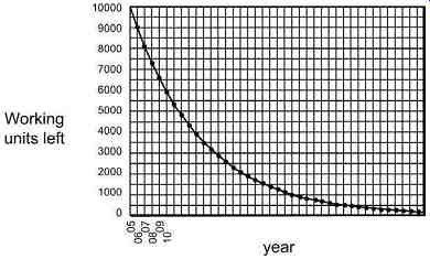
Fig. 1: How a Decaying Exponential Curve Is Naturally Generated.
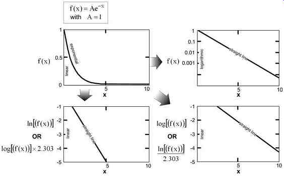
Fig. 2: Plotting the Exponential Function with a Logarithmic y-scale
or Plotting the Log of the Function with Linear y-scale - Both give a Straight
Line
Note that the simplest and most obvious initial assumption of a constant failure rate has actually led to an exponential curve. That is because the exponential curve is simply a succession of evenly spaced data points (very close to each other), that are in simple geometric progression, that is, the ratio of any point to its preceding point is a constant.
Most natural processes behave similarly, and so e is encountered very frequently.
In Fig. 2 we have plotted out a more general exponentially decaying function, of the form f(x) = A × e-x (though for simplicity, we have assumed A = 1 here). Let us now do some experiments with the way we set up the horizontal and vertical axes.
If we make the vertical scale (only) logarithmic rather than linear, we will find this gives us a straight line. Why so? That actually comes about due to a useful property of the logarithm as described next.
The definition of a logarithm is as follows - if A = BC, then log B(A) = log(C), where log B (A) is the "base-B logarithm of A." The commonly referred to "logarithm," or just "log," has an implied base of 10, whereas the natural logarithm "ln" is an abbreviation for a base-e logarithm.
So, we get the following sample relationships:
Now, if we take the natural log of both sides of the equation f (x) = A × e-x, and use the last of the equations in the previous equation set, we get ...
Further, if we compare this equation with the well-known standard equation of a straight line y(x) = mx + c (where m is the slope and c is its intersection on the y-axis), we realize that, if we plot ln f(x) on the vertical ("y") axis instead of f(x) (x being the horizontal or "x" axis), we will get a straight line.
In general, plotting a function on a log scale or plotting the log of a function on a linear scale is one and the same thing.
But what if we had plotted log f(x) on the vertical axis instead of ln f(x)? If we think about it, we realize that is the same as asking - what is the log10 of e, or equivalently, what is the loge of 10? As a matter of fact, there is not much difference really - because the base-10 and base-e logarithms are proportional to each other. This is probably more easily remembered when expressed in words - if the log of any number is multiplied by 2.303, we get its natural log. Conversely, if we divide the natural log by 2.303 we get its log. This follows from....
Therefore, plotting any arbitrary function using a log scale (base 10) will always give us the same basic "shape" as plotting the natural log of the function. And if the function is an exponential one to start with, we will get a straight line in either case (provided of course the horizontal axis is kept linear). (See Fig. 2.) Time Domain and Frequency Domain Analysis
If we have a circuit (or network) constituted only of resistors, the voltage at any point in it’s uniquely defined by the applied voltage. If the input varies, so does this voltage - instantly, and proportionally so. In other words, there is no 'lag' (delay) or 'lead' (advance) between the two. Time is not a consideration. However, when we include reactive components (capacitors and/or inductors) in any network, it becomes necessary to start looking at how the situation changes over time in response to an applied stimulus. This is called 'time domain analysis.' But we also know that any repetitive waveform, of almost arbitrary shape, can be decomposed into a sum of several sine (and cosine) waveforms of frequencies that are multiples of the basic repetition frequency 'f' ("the fundamental frequency"). That is what 'Fourier analysis' is all about. Note that though we do get an infinite series of terms, it’s composed of frequencies spaced apart from each other by an amount equal to f ; that is, we don’t get a continuum of frequencies when dealing with repetitive waveforms. But later, as we will see, when we come to more arbitrary waveshapes (nonrepetitive), we need a continuum of frequencies to decompose it.
The process of decomposition into frequency components implies that the components are mutually "independent." That is analogous to what we learn in our high-school physics class - we split a vector (applied force For example) into "orthogonal" x and y components.
We perform the math on each component considered separately, and finally sum up again to get the final vector.
In general, understanding how a system behaves with respect to the frequency components of an applied stimulus is called 'frequency domain analysis.'
Complex Representation:
A math refresher is helpful here.
We remember that the impedance of an inductor is L? and that of a capacitor is 1/C?. Here ...
? = 2pf is the angular frequency in radians/s, f being the repetition frequency (say of the Fourier component) under consideration. Since both these types of reactive components introduce a phase shift (lag or lead) between their respective voltages and currents, we can no longer just add the voltages and currents arithmetically in any circuit that contains them. The solution once again is to use a form of vector analysis, except that now, a given voltage or current vector has two components - magnitude and phase. Further, unlike a conventional vector, these components are dissimilar quantities. Therefore, we cannot use conventional vector analysis. Rather, we invoke the use of the imaginary number j = v(-1) to keep the phase and magnitude information distinct from each other, as we perform the math.
Any electrical parameter is thus written as a sum of real and imaginary parts:
A = Re + jIm
… where we have used 'Re' to denote the real part of the number A, and 'Im' its imaginary part. From these components, the actual magnitude and phase of A can be reconstructed as follows:
_ Re^2 + Im^2 (magnitude of complex number)
radians (argument of complex number)
Impedance also is broken up into a vector in this complex representation - except that though it’s frequency-dependent, it’s (usually) not a function of time.
The 'complex impedances' of reactive components are
Z = j × L?
Note that 1/j =-j. We see that the imaginary number 'j' is useful, because in effect, it also carries with it information about the 90° phase shift existing between the voltage and current in reactive components. So, the previous equations for impedance indicate that in an inductor, the current lags behind the voltage by 90°, whereas in a capacitor the current leads by the same amount. Note that resistance only has a real part, and it will therefore always be aligned with the x-axis of the complex plane (i.e. zero phase angle).
To find out what happens when a complex voltage is applied to a complex impedance, we need to apply the complex versions of our basic electrical laws. So Ohm's law, for example, now becomes:
V(?t) = I(?t) × Z(?)
We mentioned that the exponential function has some interesting properties. But a sine wave too has rather similar properties. For example, the rate of change of a sine wave is a cosine wave - which is just a sine wave phase shifted by 90?. It therefore comes as no surprise that we have the following relationships:
Note that in electrical analysis, we set ? = ?t. Here ? is the angle in radians (180° is p radians). Also, ? = 2pf , where ? is the angular frequency in radians/s and f the (conventional) frequency in Hz.
As an example, using the preceding equations, we can derive the magnitude and phase of the exponential function f (?) = ej?:
Note: Strictly speaking, a (pure) sine function is one with a phase angle of 0 and an amplitude of 1.
However, when analyzing the behavior of circuits in general, a "sine wave" is actually a sine-shaped waveform of arbitrary phase angle and magnitude. So it’s represented as AO × ej?t
- that is, with magnitude AO, and phase angle ?t (radians). For example, an applied "sine-wave" input voltage is V(t) = VO × ej?t in complex representation.
Nonrepetitive Stimuli
No stimulus is completely "repetitive" in the true sense of the word. "Repetitive" implies that the waveform has been exactly that way, since "time immemorial," and remains so forever. But in the real world, there is a definite moment when we actually apply a given waveform (and another when we remove it). Even an applied sine wave, for example, is not repetitive at the moment it gets applied at the inputs of a network. Much later, the stimulus may be considered repetitive, provided sufficient time has elapsed from the moment of application that the initial transients have died out completely. This is, in fact, the implicit assumption we always make when we carry out "steady state analysis" of a circuit.
But sometimes, we do want to know what happens at the moment of application of a stimulus - whether subsequently repetitive, steady, or otherwise. Like the case of the step voltage applied to our RC-network. If this were a power supply, for example, we would want to ensure that the output doesn't 'overshoot' (or 'undershoot') too much.
To study any such nonrepetitive waveform, we can no longer decompose it into components with discrete frequencies as we do with repetitive waveforms. Now we require a spread (continuum) of frequencies.
Further, to allow for waveforms (or frequency components) that can increase or decrease over time (disturbance changing), we need to introduce an additional (real) exponential term est. So whereas, when doing steady state analysis, we represent a sine wave in the form ej?t, now it becomes est × ej?t = e(s+j?)t . This is therefore a "sine wave," but with an exponentially increasing (s positive) or decreasing (s negative) amplitude. Note that if we are only interested in performing steady state analysis, we can go back and set s = 0.
The s-plane
In traditional ac analysis in the complex plane, the voltages and currents were complex numbers. But the frequencies were always real. However now, in an effort to include virtually arbitrary waveforms into our analysis, we have in effect created a complex frequency plane too, (s + j?). This is called s-plane, where s = s + j?. Analysis in this plane is just a more generalized form of frequency domain analysis.
[...]
This looks like a parallel combination (for resistors and inductors), but in reality, it’s a series combination (of capacitors).
To calculate the response of complex circuits and stimuli in the s-plane, we will need to use the above impedance summing rules, along with the rather obvious s-plane versions of the electrical laws. For example, Ohm's law is now:
V(s) = I(s) × Z(s)
Finally, the use of s gives us the ability to solve the differential equations arising from an almost arbitrary stimulus, in an elegant way, as opposed to the brute-force method in the time domain. The technique used to do this is the ' Laplace transform.' Note: Any such decomposition method can be practical only when we are dealing with "mathematical" waveforms. Real waveforms may need to be approximated by known mathematical functions for further analysis. And very arbitrary waveforms will probably prove intractable.
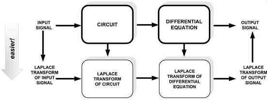
Fig. 3: Symbolic Representation of the Procedure for Working in the S-plane