Electric Machinery--Speed and Torque Control

The objective of this section is to discuss various techniques for the control of electric machines. Since an in-depth discussion of this topic is both too extensive for a single section and beyond the scope of this guide, the presentation here will necessarily be introductory in nature. We will present basic techniques for speed and torque control and will illustrate typical configurations of drive electronics that are used to implement the control algorithms. This section will build upon the discussion of power electronics in Section 10.

Note that the discussion of this section is limited to steady-state operation. The steady-state picture presented here is quite adequate for a wide variety of electric-machine applications. However, the reader is cautioned that system dynamics can play a critical role in some applications, with concerns ranging from speed of response to overall system stability. Although the techniques presented here form the basis for dynamic analyses, the constraints of an introductory textbook are such that a more extensive discussion, including transient and dynamic behavior, is not possible.

In the discussion of torque control for synchronous and induction machines, the techniques of field-oriented or vector control are introduced and the analogy is made with torque control in dc motors. This material is somewhat more sophisticated mathematically than the speed-control discussion and requires application of the dq0 transformations developed in Section C. The section is written such that this material can be omitted at the discretion of the instructor without detracting from the discussion of speed control.

1. CONTROL OF DC MOTORS

Before the widespread application of power-electronic drives to control ac machines, dc motors were by far the machines of choice in applications requiring flexibility of control. Although in recent years ac drives have become quite common, the ease of control of dc machines insure their continued use in many applications.

1.1 Speed Control

The three most common speed-control methods for dc motors are adjustment of the flux, usually by means of field-current control, adjustment of the resistance associated with the armature circuit, and adjustment of the armature terminal voltage.

Field-Current Control

In part because it involves control at a relatively low power level (the power into the field winding is typically a small fraction of the power into the armature of a dc machine), field-current control is frequently used to control the speed of a dc motor with separately excited or shunt field windings. The equivalent circuit for a separately excited dc machine is found in Fig. 7.4a and is repeated in FIG. 1. The method is, of course, also applicable to compound motors. The shunt field current can be adjusted by means of a variable resistance in series with the shunt field. Alternatively, the field current can be supplied by power-electronic circuits which can be used to rapidly change the field current in response to a wide variety of control signals.

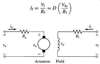
FIG. 1 Equivalent circuit for a separately excited dc motor.

FIG. 2a shows in schematic form a switching scheme for pulse-width modulation of the field voltage. This system closely resembles the pulse-width modulation system discussed in Section 10.3.2. It consists of a rectifier which rectifies the ac input voltage, a dc-link capacitor which filters the rectified voltage, producing a dc voltage Vdc, and a pulse-width modulator.

In this system, because only a unidirectional field current is required, the pulsewidth modulator consists of a single switch and a free-wheeling diode rather than the more complex four-switch arrangement of Fig. 10.45. Assuming both the switch and diode to be ideal, the average voltage across the field winding will be equal to

(Eq. 1)

...where D is the duty cycle of the switching waveform; i.e., D is the fraction of time that the switch S is on.

FIG. 2b shows the resultant field current. Because in the steady-state the average voltage across the inductor must equal zero, the average field current If will thus be equal to

(Eq. 2)

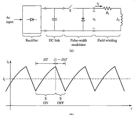
FIG. 2 (a) Pulse-width modulation system for a dc-machine field winding. (b) Field-current waveform.

Thus, the field current can be controlled simply by controlling the duty cycle of the pulse-width modulator. If the field-winding time constant Lf/Rf is long compared to the switching time, the ripple current Aif will be small compared to the average current If.

Armature-Circuit Resistance Control

Armature-circuit resistance control provides a means of obtaining reduced speed by the insertion of external series resistance in the armature circuit. It can be used with series, shunt, and compound motors; for the last two types, the series resistor must be connected between the shunt field and the armature, not between the line and the motor. It is a common method of speed control for series motors and is generally analogous in action to wound-rotor-induction-motor control by the addition of external series rotor resistance.

Depending upon the value of the series armature resistance, the speed may vary significantly with load, since the speed depends on the voltage drop in this resistance and hence on the armature current demanded by the load. For example, a 1200-r/min shunt motor whose speed under load is reduced to 750 r/min by series armature resistance will return to almost 1200-r/min operation if the load is removed because the no-load current produces a voltage drop across the series resistance which is insignificant. The disadvantage of poor speed regulation may not be important in a series motor, which is used only where varying-speed service is required or can be tolerated.

A significant disadvantage of this method of speed control is that the power loss in the external resistor is large, especially when the speed is greatly reduced. In fact, for a constant-torque load, the power input to the motor plus resistor remains constant, while the power output to the load decreases in proportion to the speed. Operating costs are therefore comparatively high for lengthy operation at reduced speeds. Because of its low initial cost however, the series-resistance method (or the variation of it discussed in the next paragraph) will often be attractive economically for applications which require only short-time or intermittent speed reduction. Unlike field-current control, armature-resistance control results in a constant-torque drive because both the field-flux and, to a first approximation, the allowable armature current remain constant as speed changes.

A variation of this control scheme is given by the shunted-armature method, which may be applied to a series motor, as in FIG. 3a, or a shunt motor, as in FIG. 3b. In effect, resistors R1 and R2 act as a voltage divider applying a reduced voltage to the armature. Greater flexibility is possible because two resistors can now be adjusted to provide the desired performance. For series motors, the no-load speed can be adjusted to a finite, reasonable value, and the scheme is therefore applicable to the production of slow speeds at light loads. For shunt motors, the speed regulation in the low-speed range is appreciably improved because the no-load speed is definitely lower than the value with no controlling resistors.

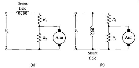
FIG. 3 Shunted-armature method of speed control applied to (a) a series motor and (b) a shunt motor.

Armature-Terminal Voltage Control

Armature-terminal voltage control can be readily accomplished with the use of power-electronic systems such as those discussed in Section 10. FIG. 4 shows in somewhat schematic form three possible configurations. In FIG. 4a, a phase-controlled rectifier in combination with a dc link filter capacitor can be used to produce a variable dc-link voltage which can be applied directly to the armature terminals of the dc motor.

In FIG. 4b, a constant dc-link voltage is produced by a diode rectifier in combination with a dc-link filter capacitor. The armature terminal voltage is then varied by a pulse-width modulation scheme in which switch S is alternately opened and closed.

When switch S is closed, the armature voltage is equal to the dc-link voltage Vdc, and when the switch is opened, current transfers to the freewheeling diode, essentially setting the armature voltage to zero. Thus the average armature voltage under this condition is equal to

Va = D Vdc (Eq. 7)

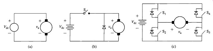
FIG. 4 Three typical configurations for armature-voltage control. (a) Variable dc-link voltage (produced by a phase-controlled rectifier) applied directly to the dc-motor armature terminals. (b) Constant dc-link voltage with single-polarity pulse-width modulation. (c) Constant dc-link voltage with a full H-bridge.

where

Va = average armature voltage (V)

Vdc = dc-link voltage (V)

D = PWM duty cycle (fraction of time that switch S is closed)

FIG. 4c shows an H-bridge configuration as is discussed in the context of inverters in Section 10.3.3. Note that if switch $3 is held closed while switch $4 remains open, this configuration reduces to that of FIG. 4b. However, the H-bridge configuration is more flexible because it can produce both positive- and negative-polarity armature voltage. For example, with switches S1 and S3 closed, the armature voltage is equal to V~c while with switches S2 and S4 closed, the armature voltage is equal to -Vdc. Clearly, using such an H-bridge configuration in combination with an appropriate choice of control signals to the switches allows this PWM system to achieve any desired armature voltage in the range -V~c < Va < V~c.

Armature-voltage control takes advantage of the fact that, because the voltage drop across the armature resistance is relatively small, a change in the armature terminal voltage of a shunt motor is accompanied in the steady state by a substantially equal change in the speed voltage. With constant shunt field current and hence field flux, this change in speed voltage must be accompanied by a proportional change in motor speed. Thus, motor speed can be controlled directly by means of the armature terminal voltage.

-------------

Practice Problem 3

Calculate the change in armature voltage required to maintain the motor of Example 3 at a speed of 2000 r/min as the load is changed from zero to full-load torque.

Solution

12.5 V

-------------

Frequently the control of motor voltage is combined with field-current control in order to achieve the widest possible speed range. With such dual control, base speed can be defined as the normal-armature-voltage, full-field speed of the motor.

Speeds above base speed are obtained by reducing the field current; speeds below base speed are obtained by armature-voltage control. As discussed in connection with field-current control, the range above base speed is that of a constant-power drive.

The range below base speed is that of a constant-torque drive because, as in armature-resistance control, the flux and the allowable armature current remain approximately constant. The overall output limitations are therefore as shown in FIG. 6a for approximate allowable torque and in FIG. 6b for approximate allowable power.

The constant-torque characteristic is well suited to many applications in the machine-tool industry, where many loads consist largely of overcoming the friction of moving parts and hence have essentially constant torque requirements.

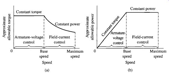
FIG. 6 (a) Torque and (b) power limitations of combined armature-voltage and field-current methods of speed control.

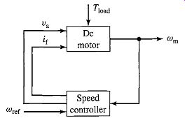
FIG. 7 Block diagram for a speed-control system for a separately excited or shunt-connected dc motor.

The speed regulation and the limitations on the speed range above base speed are those already presented with reference to field-current control; the maximum speed thus does not ordinarily exceed four times base speed and preferably not twice base speed. For conventional machines, the lower limit for reliable and stable operation is about one-tenth of base speed, corresponding to a total maximum-to-minimum range not exceeding 40:1.

With armature reaction ignored, the decrease in speed from no-load to full-load torque is caused entirely by the full-load armature-resistance voltage drop in the dc generator and motor. This full-load armature-resistance voltage drop is constant over the voltage-control range, since full-load torque and hence full-load current are usually regarded as constant in that range. When measured in r/min, therefore, the speed decrease from no-load to full-load torque is a constant, independent of the no-load speed, as we saw in Example 3. The torque-speed curves accordingly are closely approximated by a series of parallel straight lines for the various motor-field adjustments. Note that a speed decrease of, say, 40 r/min from a no-load speed of 1200 r/min is often of little importance; a decrease of 40 r/min from a no-load speed of 120 r/min, however, may at times be of critical importance and require corrective steps in the layout of the system.

FIG. 7 shows a block diagram of a feedback-control system that can be used to regulate the speed of a separately excited or shunt-connected dc motor. The inputs to the dc-motor block include the armature voltage and the field current as well as the load torque T_load. The resultant motor speed O)m is fed back to a controller block which represents both the control logic and power electronics and which controls the armature voltage and field current applied to the dc motor, based upon a reference speed signal O)ref. Depending upon the design of the controller, with such a scheme it is possible to control the steady-state motor speed to a high degree of accuracy independent of the variations in the load torque.

1.2 Torque Control

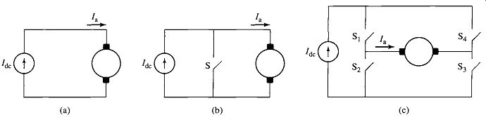
FIG. 9 Three typical configurations for armature-current control. (a) Variable dc-link current (produced by a phase-controlled rectifier) applied directly to the dc-motor armature terminals. (b) Constant dc-link current with single-polarity pulse-width modulation. (c) Constant dc-link current with a full H-bridge.

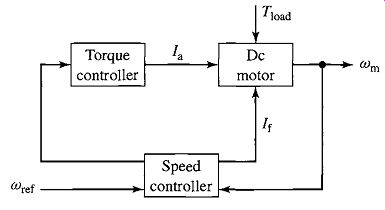
FIG. 10 Block diagram of a dc-motor speed-control system using direct-control of motor torque.

As we have seen, the electromagnetic torque of a dc motor is proportional to the armature current la and is given by:

(Eq. 10)

... in the case of a separately excited or shunt motor and ...

(Eq. 11)

... in the case of a permanent-magnet motor.

From these equations we see that torque can be controlled directly by controlling the armature current. FIG. 9 shows three possible configurations. In FIG. 9a, a phase-controlled rectifier, in combination with a dc-link filter inductor, can be used to create a variable dc-link current which can be applied directly to the armature terminals of the dc motor.

In FIG. 9b, a constant dc-link current is produced by a diode rectifier. The armature terminal voltage is then varied by a pulse-width modulation scheme in which switch S is alternately opened and closed. When switch S is opened, the current Idc flows into the dc-motor armature while when switch S is closed, the armature is shorted and Ia decays. Thus, the duty cycle of switch S will control the average current into the armature.

Finally, Fig 9c shows an H-bridge configuration as is discussed in the context of inverters in Section 10.3.2. Appropriate control of the four switches S 1 through S4 allows this PWM system to achieve any desired armature average current in the range--Idc < Ia < /de.

Note that in each of the PWM configurations of FIG. 9b and c, rapid changes in instantaneous current through the dc machine armature can give rise to large voltage spikes, which can damage the machine insulation as well as give rise to flashover and voltage breakdown of the commutator. In order to eliminate these effects, a practical system must include some sort of filter across the armature terminals (such as a large capacitor) to limit the voltage rise and to provide a low-impedance path for the high-frequency components of the drive current.

FIG. 10 shows a typical configuration in which the torque control is surrounded by a speed-feedback loop. This looks similar to the speed control of FIG. 7. However, instead of controlling the armature voltage, in this case the output of the speed controller is a torque reference signal Tref which in turn serves as the input to the torque controller. One advantage of such a system is that it automatically limits the dc-motor armature current to acceptable levels under all operating conditions, as is shown in Example 6.

2. CONTROL OF SYNCHRONOUS MOTORS

2.1 Speed Control

As discussed in Sections 4 and 5, synchronous motors are essentially constant-speed machines, with their speed being determined by the frequency of the armature currents as described by Eqs. 4.40 and 4.41. Specifically, Eq. 4.40 shows that the synchronous angular velocity is proportional to the electrical frequency of the applied armature voltage and inversely proportional to the number of poles in the machine

(Eq. 12)

... where:

cos = synchronous spatial angular velocity of the air-gap mmf wave [rad/sec]

COe = 2n'fe = angular frequency of the applied electrical excitation [rad/sec]

fe = applied electrical frequency [Hz]

Clearly, the simplest means of synchronous motor control is speed control via control of the frequency of the applied armature voltage, driving the motor by a polyphase voltage-source inverter such as the three-phase inverter shown in FIG. 11. As is discussed in Section 10.3.3, this inverter can either be used to supply stepped ac voltage waveforms of amplitude V, tc or the switches can be controlled to produce pulse-width-modulated ac voltage waveforms of variable amplitude. The dc-link voltage Vdc can itself be varied, for example, through the use of a phase-controlled rectifier.

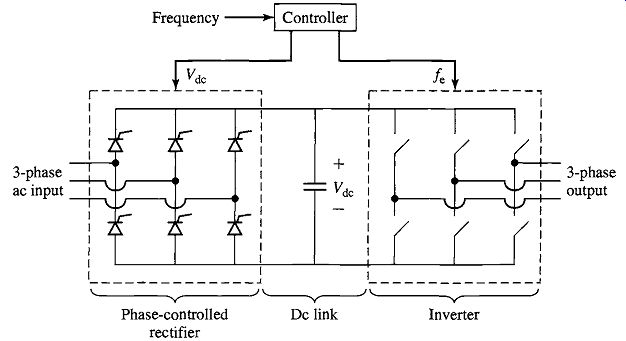
FIG. 11 Three-phase voltage-source inverter.

The frequency of the inverter output waveforms can of course be varied by controlling the switching frequency of the inverter switches. For ac-machine applications, coupled with this frequency control must be control of the amplitude of the applied voltage, as we will now see.

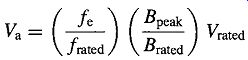
From Faraday's Law, we know that the air-gap component of the armature voltage in an ac machine is proportional to the peak flux density in the machine and the electrical frequency. Thus, if we neglect the voltage drop across the armature resistance and leakage reactance, we can write:

(Eq. 13)

... where Va is the amplitude of the armature voltage, fe is the operating frequency, and Bpeak is the peak air-gap flux density. V_rated, f_rated, and B_rated are the corresponding rated-operating-point values.

Consider a situation in which the frequency of the armature voltage is varied while its amplitude is maintained at its rated value (Va = Vrated). Under these conditions, from Eq. 13 we see that:

(Eq. 14)

Equation 14 clearly demonstrates the problem with constant-voltage, variable frequency operation. Specifically, for a given armature voltage, the machine flux density is inversely proportional to frequency and thus as the frequency is reduced, the flux density will increase. Thus for a typical machine which operates in saturation at rated voltage and frequency, any reduction in frequency will further increase the flux density in the machine. In fact, a significant drop in frequency will increase the flux density to the point of potential machine damage due both to increased core loss and to the increased machine currents required to support the higher flux density.

As a result, for frequencies less than or equal to rated frequency, it is typical to operate a machine at constant flux density. From Eq. 13, with Bpeak = Brated

(Eq. 15)

.....which can be rewritten as ........

(Eq. 16)

From Eq. 16, we see that constant-flux operation can be achieved by maintaining a constant ratio of armature voltage to frequency. This is referred to as constant volts-per-hertz (constant V/Hz) operation. It is typically maintained from rated frequency down to the low frequency at which the armature resistance voltage drop becomes a significant component of the applied voltage.

Similarly, we see from Eq. 13 that if the machine is operated at frequencies in excess of rated frequency with the voltage at its rated value, the air-gap flux density will drop below its rated value. Thus, in order to maintain the flux density at its rated value, it would be necessary to increase the terminal voltage for frequencies in excess of rated frequency. In order to avoid insulation damage, it is common to maintain the machine terminal voltage at its rated value for frequencies in excess of rated frequency.

The machine terminal current is typically limited by thermal constraints. Thus, provided the machine cooling is not affected by rotor speed, the maximum permissible terminal current will remain constant at its rated value/rated, independent of the applied frequency. As a result, for frequencies below rated frequency, with Va proportional to fe, the maximum machine power will be proportional to fe Vrated/rated. The maximum torque under these conditions can be found by dividing the power by the rotor speed COs, which is also proportional to fe as can be seen from Eq. 12. Thus, we see that the maximum torque is proportional to Vrated/rated, and hence it is constant at its rated-operating-point value.

Similarly, for frequencies in excess of rated frequency, the maximum power will be constant and equal to Vrated / rated . The corresponding maximum torque will then vary inversely with machine speed as Vrated/rated/COs . The maximum operating speed for this operating regime will be determined either by the maximum frequency which can be supplied by the drive electronics or by the maximum speed at which the rotor can be operated without risk of damage due to mechanical concerns such as excessive centrifugal force or to the presence of a resonance in the shaft system.

FIG. 12 shows a plot of maximum power and maximum torque versus speed for a synchronous motor under variable-frequency operation. The operating regime below rated frequency and speed is referred to as the constant-torque regime and that above rated speed is referred to as the constant-power regime.

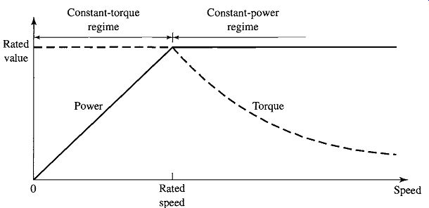
FIG. 12 Variable-speed operating regimes for a synchronous motor.

Although during steady-state operation the speed of a synchronous motor is determined by the frequency of the drive, speed control by means of frequency control is of limited use in practice. This is due in most part to the fact that it is difficult for the rotor of a synchronous machine to track arbitrary changes in the frequency of the applied armature voltage. In addition, starting is a major problem, and, as a result, the rotors of synchronous motors are often equipped with a squirrel-cage winding known as an amortisseur or damper winding similar to the squirrel-cage winding in an induction motor, as shown in Fig. 5.3. Following the application of a polyphase voltage to the armature, the rotor will come up almost to synchronous speed by induction-motor action with the field winding unexcited. If the load and inertia are not too great, the motor will pull into synchronism when the field winding is subsequently energized.

Problems with changing speed result from the fact that, in order to develop torque, the rotor of a synchronous motor must remain in synchronism with the stator flux.

Control of synchronous motors can be greatly enhanced by control algorithms in which the stator flux and its relationship to the rotor flux are controlled directly. Such control, which amounts to direct control of torque, is discussed in Sect. 2.2.

2.2 Torque Control

Direct torque control in an ac machine, which can be implemented in a number of different ways, is commonly referred to as field-oriented control or vector control. To facilitate our discussion of field-oriented control, it is helpful to return to the discussion of Section 5.6.1. Under this viewpoint, which is formalized in Section C, stator quantities (flux, current, voltage, etc.) are resolved into components which rotate in synchronism with the rotor. Direct-axis quantities represent those components which are aligned with the field-winding axis, and quadrature-axis components are aligned perpendicular to the field-winding axis.

Section C.2 of Section C derives the basic machine relations in dq0 variables for a synchronous machine consisting of a field winding and a three-phase stator winding. The transformed flux-current relationships are found to be:

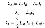
(Eq. 17)

(Eq. 18)

(Eq. 19)

where the subscripts d, q, and f refer to armature direct-, quadrature-axis, and field winding quantities respectively. Note that throughout this section we will assume balanced operating conditions, in which case zero-sequence quantities will be zero and hence will be ignored.

The corresponding transformed voltage equations are:

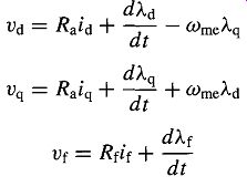
(Eq. 20)

(Eq. 21)

(Eq. 22)

where (-Ome -(poles/2)Wm is the electrical angular velocity of the rotor.

[....]

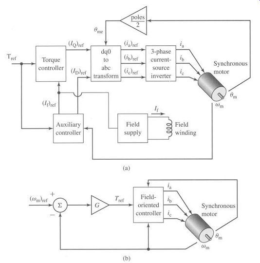
FIG. 13 (a) Block diagram of a field-oriented torque-control system for a synchronous motor. (b) Block diagram of a synchronous-motor speed-control loop built around a field-oriented torque control system.

3. CONTROL OF INDUCTION MOTORS

3.1 Speed Control

Induction motors supplied from a constant-frequency source admirably fulfill the requirements of substantially constant-speed drives. Many motor applications, however, require several speeds or even a continuously adjustable range of speeds. From the earliest days of ac power systems, engineers have been interested in the development of adjustable-speed ac motors.

The synchronous speed of an induction motor can be changed by (a) changing the number of poles or (b) varying the line frequency. The operating slip can be changed by (c) varying the line voltage, (d) varying the rotor resistance, or (e) applying voltages of the appropriate frequency to the rotor circuits. The salient features of speed-control methods based on these five possibilities are discussed in the following five sections.

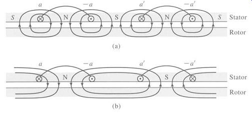
FIG. 16 Principles of the pole-changing winding.

Pole-Changing Motors

In pole-changing motors, the stator winding is designed so that, by simple changes in coil connections, the number of poles can be changed in the ratio 2 to 1. Either of two synchronous speeds can then be selected. The rotor is almost always of the squirrel-cage type, which reacts by producing a rotor field having the same number of poles as the inducing stator field. With two independent sets of stator windings, each arranged for pole changing, as many as four synchronous speeds can be obtained in a squirrel-cage motor, for example, 600, 900, 1200, and 1800 r/min for 60-Hz operation.

The basic principles of the pole-changing winding are shown in FIG. 16, in which aa and a'a' are two coils comprising part of the phase-a stator winding. An actual winding would, of course, consist of several coils in each group. The windings for the other stator phases (not shown in the figure) would be similarly arranged. In FIG. 16a the coils are connected to produce a four-pole field; in FIG. 16b the current in the a'a' coil has been reversed by means of a controller, the result being a two-pole field.

FIG. 17 shows the four possible arrangements of these two coils: they can be connected in series or in parallel, and with their currents either in the same direction (four-pole operation) or in the opposite direction (two-pole operation). Additionally, the machine phases can be connected either in Y or A, resulting in eight possible combinations.

Note that for a given phase voltage, the different connections will result in differing levels of air-gap flux density. For example, a change from a A to a Y connection will reduce the coil voltage (and hence the air-gap flux density) for a given coil arrangement by ~. Similarly, changing from a connection with two coils in series to two in parallel will double the voltage across each coil and therefore double the magnitude of the air-gap flux density. These changes in flux density can, of course, be compensated for by changes in the applied winding voltage. In any case, they must be considered, along with corresponding changes in motor torque, when the configuration to be used in a specific application is considered.

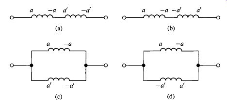
FIG. 17 Four possible arrangements of phase-a stator coils in a pole-changing induction motor: (a) series-connected, four-pole; (b) series-connected, two-pole; (c)parallel-connected, four-pole; (d) parallel-connected, two-pole.

Armature-Frequency Control

The synchronous speed of an induction motor can be controlled by varying the frequency of the applied armature voltage. This method of speed control is identical to that discussed in Sect. 2.1 for synchronous machines. In fact, the same inverter configurations used for synchronous machines, such as the three-phase voltage-source inverter of FIG. 11, can be used to drive induction motors. As is the case with any ac motor, to maintain approximately constant flux density, the armature voltage should also be varied directly with the frequency (constant-volts-per-hertz). The torque-speed curve of an induction motor for a given frequency can be calculated by using the methods of Section 6 within the accuracy of the motor parameters at that frequency. Consider the torque expression of Eq. 6.33 which is repeated here.

[...]

Line-Voltage Control

The internal torque developed by an induction motor is proportional to the square of the voltage applied to its primary terminals, as shown by the two torque-speed characteristics in FIG. 19. If the load has the torque-speed characteristic shown by the dashed line, the speed will be reduced from n1 to n2. This method of speed control is commonly used with small squirrel-cage motors driving fans, where cost is an issue and the inefficiency of high-slip operation can be tolerated.

It is characterized by a rather limited range of speed control.

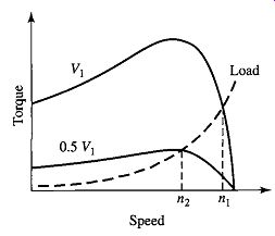
FIG. 19 Speed control by means of line voltage.

Rotor-Resistance Control

The possibility of speed control of a wound-rotor motor by changing its rotor-circuit resistance has already been pointed out in Section 6.7.1.

The torque-speed characteristics for three different values of rotor resistance are shown in FIG. 20. If the load has the torque-speed characteristic shown by the dashed line, the speeds corresponding to each of the values of rotor resistance are n1, n2, and n3. This method of speed control has characteristics similar to those of dc shunt-motor speed control by means of resistance in series with the armature.

The principal disadvantages of both line-voltage and rotor-resistance control are low efficiency at reduced speeds and poor speed regulation with respect to change in load. In addition, the cost and maintenance requirements of wound-rotor induction motors are sufficiently high that squirrel-cage motors combined with solid-state drives have become the preferred option in most applications.

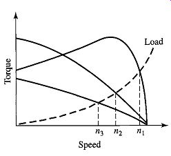
FIG. 20 Speed control by means of rotor resistance.

3.2 Torque Control

In Sect. 2.2 we developed the concept of field-oriented-control for synchronous machines. Under this viewpoint, the armature flux and current are resolved into two components which rotate synchronously with the rotor and with the air-gap flux wave.

The components of armature current and flux which are aligned with the field-winding are referred to as direct-axis components while those which are perpendicular to this axis are referred to as quadrature-axis components.

It turns out that the same viewpoint which we applied to synchronous machines can be applied to induction machines. As is discussed in Section 6.1, in the steadystate the mmf and flux waves produced by both the rotor and stator windings of an induction motor rotate at synchronous speed and in synchronism with each other.

Thus, the torque-producing mechanism in an induction machine is equivalent to that of a synchronous machine. The difference between the two is that, in an induction machine, the rotor currents are not directly supplied but rather are induced as the induction-motor rotor slips with respect to the rotating flux wave produced by the stator currents.

To examine the application of field-oriented control to induction machines, we begin with the dq0 transformation of Section C.3 of Section C. This transformation transforms both the stator and rotor quantities into a synchronously rotating reference frame. Under balanced-three-phase, steady-state conditions, zero-sequence quantities will be zero and the remaining direct- and quadrature-axis quantites will be constant.

Hence the flux-linkage current relationships of Eqs. C.52 through C.58 become [...]

4. CONTROL OF VARIABLE-RELUCTANCE MOTORS

Unlike dc and ac (synchronous or induction) machines, VRMs cannot be simply "plugged in" to a dc or ac source and then be expected to run. As is discussed in Section 8, the phases must be excited with (typically unipolar) currents, and the timing of these currents must be carefully correlated with the position of the rotor poles in order to produce a useful, time-averaged torque. The result is that although the VRM itself is perhaps the simplest of rotating machines, a practical VRM drive system is relatively complex.

VRM drive systems are competitive only because this complexity can be realized easily and inexpensively through power and microelectronic circuitry. These drive systems require a fairly sophisticated level of controllability for even the simplest modes of VRM operation. Once the capability to implement this control is available, fairly sophisticated control features can be added (typically in the form of additional software) at little additional cost, further increasing the competitive position of VRM drives.

In addition to the VRM itself, the basic VRM drive system consists of the following components: a rotor-position sensor, a controller, and an inverter. The function of the rotor-position sensor is to provide an indication of shaft position which can be used to control the timing and waveform of the phase excitation. This is directly analogous to the timing signal used to control the firing of the cylinders in an automobile engine.

The controller is typically implemented in software in microelectronic (microprocessor) circuitry. Its function is to determine the sequence and waveforms of the phase excitation required to achieve the desired motor speed-torque characteristics. In addition to set points of desired speed and/or torque and shaft position (from the shaft position sensor), sophisticated controllers often employ additional inputs including shaft-speed and phase-current magnitude. Along with the basic control function of determining the desired torque for a given speed, the more sophisticated controllers attempt to provide excitations which are in some sense optimized (for maximum efficiency, stable transient behavior, etc.). The control circuitry consists typically of low-level electronics which cannot be used to directly supply the currents required to excite the motor phases. Rather its output consists of signals which control an inverter which in turn supplies the phase currents. Control of the VRM is achieved by the application of an appropriate set of currents to the VRM phase windings.

Figures 11.23a to c show three common configurations found in inverter systems for driving VRMs. Note that these are simply H-bridge inverters of the type discussed in Section 10.3. Each inverter is shown in a two-phase configuration. As is clear from the figures, extension of each configuration to drive additional phases can be readily accomplished.

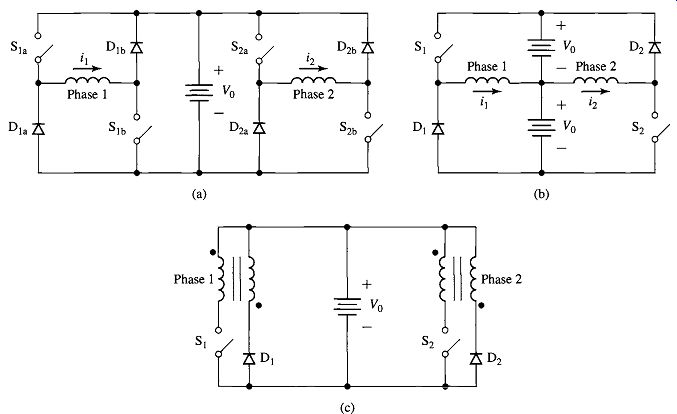
FIG. 23 Inverter configurations. (a) Two-phase inverter which uses two switches per phase. (b) Two-phase inverter which uses a split supply and one switch per phase. (c) Two-phase inverter with bifilar phase windings and one switch per phase.

The configuration of FIG. 23a is perhaps the simplest. Closing switches Sla and Slb connects the phase-1 winding across the supply (V1 = V0) and causes the winding current to increase. Opening just one of the switches forces a short across the winding and the current will decay, while opening both switches connects the winding across the supply with negative polarity through the diodes (Vl = -V0) and the winding current will decay more rapidly. Note that this configuration is capable of regeneration (returning energy to the supply), but not of supplying negative current to the phase winding. However, since the torque in a VRM is proportional to the square of the phase current, there is no need for negative winding current.

As discussed in Section 10.3.2, the process of pulse-width modulation, under which a series of switch configurations alternately charge and discharge a phase winding, can be used to control the average winding current. Using this technique, an inverter such as that of FIG. 23a can readily be made to supply the range of waveforms required to drive a VRM. The inverter configuration of FIG. 23a is perhaps the simplest of H-bridge configurations which provide regeneration capability. Its main disadvantage is that it requires two switches per phase. In many applications, the cost of the switches (and their associated drive circuitry) dominates the cost of the inverter, and the result is that this configuration is less attractive in terms of cost when compared to other configurations which require one switch per phase.

FIG. 23b shows one such configuration. This configuration requires a split supply (i.e., two supplies of voltage V0) but only a single switch and diode per phase.

Closing switch S1 connects the phase-1 winding to the upper dc source. Opening the switch causes the phase current to transfer to diode D1, connecting the winding to the bottom dc source. Phase 1 is thus supplied by the upper dc source and regenerates through the bottom source. Note that to maintain symmetry and to balance the energy supplied from each source equally, phase 2 is connected oppositely so that it is supplied from the bottom source and regenerates into the top source.

The major disadvantages of the configuration of FIG. 23b are that it requires a split supply and that when the switch is opened, the switch must withstand a voltage of 2 V0. This can be readily seen by recognizing that when diode D1 is forward-biased, the switch is connected across the two supplies. Such switches are likely to be more expensive than the switches required by the configuration of FIG. 23a. Both of these issues will tend to offset some of the economic advantage which can be gained by the elimination of one switch and one diode as compared with the inverter circuit of FIG. 23a.

A third inverter configuration is shown in FIG. 23c. This configuration requires only a single dc source and uses only a single switch and diode per phase. This configuration achieves regeneration through the use of bifilar phase windings. In a bifilar winding, each phase is wound with two separate windings which are closely coupled magnetically (this can be achieved by winding the two windings at the same time) and can be thought of as the primary and secondary windings of a transformer.

When switch S1 is closed, the primary winding of phase 1 is energized, exciting the phase winding. Opening the switch induces a voltage in the secondary winding (note the polarity indicated by the dots in FIG. 23c) in such a direction as to forward bias D1. The result is that current is transferred from the primary to the secondary winding with a polarity such that the current in the phase decays to zero and energy is returned to the source.

Although this configuration requires only a single dc source, it requires a switch which must withstand a voltage in excess of 2V0 (the degree of excess being determined by the voltage developed across the primary leakage reactance as current is switched from the primary to the secondary windings) and requires the more complex bifilar winding in the machine. In addition, the switches in this configuration must include snubbing circuitry (typically consisting of a resistor-capacitor combination) to protect them from transient overvoltages. These overvoltages result from the fact that although the two windings of the bifilar winding are wound such that they are as closely coupled as possible, perfect coupling cannot be achieved. As a result, there will be energy stored in the leakage fields of the primary winding which must be dissipated when the switch is opened.

As is discussed in Section 10.3, VRM operation requires control of the current applied to each phase. For example, one control strategy for constant torque production is to apply constant current to each phase during the time that dL/d Om for that phase is constant. This results in constant torque proportional to the square of the phase-current magnitude. The magnitude of the torque can be controlled by changing the magnitude of the phase current.

The control required to drive the phase windings of a VRM is made more complex because the phase-winding inductances change both with rotor position and with current levels due to saturation effects in the magnetic material. As a result, it is not possible in general to implement an open-loop PWM scheme based on a precalculated algorithm. Rather, pulse-width-modulation is typically accomplished through the use of current feedback. The instantaneous phase current can be measured and a switching scheme can be devised such that the switch can be turned off when the current has been found to reach a desired maximum value and turned on when the current decays to a desired minimum value. In this manner the average phase current is controlled to a predetermined function of the rotor position and desired torque.

This section has provided a brief introduction to the topic of drive systems for variable-reluctance machines. In most cases, many additional issues must be considered before a practical drive system can be implemented. For example, accurate rotor-position sensing is required for proper control of the phase excitation, and the control loop must be properly compensated to ensure its stability. In addition, the finite rise and fall times of current buildup in the motor phase windings will ultimately limit the maximum achievable rotor torque and speed.

The performance of a complete VRM drive system is intricately tied to the performance of all its components, including the VRM, its controller, and its inverter.

In this sense, the VRM is quite different from the induction, synchronous, and dc machines discussed earlier in this section. As a result, it is useful to design the complete drive system as an integrated package and not to design the individual components (VRM, inverter, controller, etc.) separately. The inverter configurations of FIG. 23 are representative of a number of possible inverter configurations which can be used in VRM drive systems. The choice of an inverter for a specific application must be made based on engineering and economic considerations as part of an integrated VRM drive system design.

5. SUMMARY

This section introduces various techniques for the control of electric machines. The broad topic of electric machine control requires a much more extensive discussion than is possible here so our objectives have been somewhat limited. Most noticeably, the discussion of this section focuses almost exclusively on steady-state behavior, and the issues of transient and dynamic behavior are not considered.

Much of the control flexibility that is now commonly associated with electric machinery comes from the capability of the power electronics that is used to drive these machines. This section builds therefore on the discussion of power electronics in Section 10.

The starting point is a discussion of dc motors for which it is convenient to subdivide the control techniques into two categories: speed and torque control. The algorithm for speed control in a dc motor is relatively straight forward. With the exception of a correction for voltage drop across the armature resistance, the steady state speed is determined by the condition that the generated voltage must be equal to the applied armature voltage. Since the generated voltage is proportional to the field flux and motor speed, we see that the steady-state motor speed is proportional to the armature voltage and inversely proportional to the field flux.

An alternative viewpoint is that of torque control. Because the commutator/brush system maintains a constant angular relationship between the field and armature flux, the torque in a dc motor is simply proportional to the product of the armature current and the field flux. As a result, dc motor torque can be controlled directly by controlling the armature current as well as the field flux.

Because synchronous motors develop torque only at synchronous speed, the speed of a synchronous motor is simply determined by the electrical frequency of the applied armature excitation. Thus, steady-state speed control is simply a matter of armature frequency control. Torque control is also possible. By transforming the stator quantities into a reference frame rotating synchronously with the rotor (using the dq0 transformation of Section C), we found that torque is proportional to the field flux and the component of armature current in space quadrature with the field flux. This is directly analogous to the torque production in a dc motor. Control schemes which adopt this viewpoint are referred to as vector or field-oriented control.

Induction machines operate asynchronously; rotor currents are induced by the relative motion of the rotor with respect to the synchronously rotating stator-produced flux wave. When supplied by a constant-frequency source applied to the armature winding, the motor will operate at a speed somewhat lower than synchronous speed, with the motor speed decreasing as the load torque is increased. As a result, precise speed regulation is not a simple matter, although in most cases the speed will not vary from synchronous speed by an excessive amount.

Analogous to the situation in a synchronous motor, in spite of the fact that the rotor of an induction motor rotates at less than synchronous speed, the interaction between the rotor and stator flux waves is indeed synchronous. As a result, a transformation into a synchronously rotating reference frame results in rotor and stator flux waves which are constant. The torque can then be expressed in terms of the product of the rotor flux linkages and the component of armature current in quadrature with the rotor flux linkages (referred to as the quadrature-axis component of the armature current) in a fashion directly analogous to the field-oriented viewpoint of a synchronous motor. Furthermore, it can be shown that the rotor flux linkages are proportional to the direct-axis component of the armature current, and thus the direct-axis component of armature current behaves much like the field current in a synchronous motor. This field-oriented viewpoint of induction machine control, in combination with the power-electronic and control systems required to implement it, has led to the widespread applicability of induction machines to a wide range of variable-speed applications.

Finally, this section ends with a brief discussion of the control of variable reluctance machines. To produce useful torque, these machines typically require relatively complex, nonsinusoidal current waveforms whose shape must be controlled as a function of rotor position. Typically, these waveforms are produced by pulse-width modulation combined with current feedback using an H-bridge inverter of the type discussed in Section 10. The details of these waveforms depend heavily upon the geometry and magnetic properties of the VRM and can vary significantly from motor to motor.

6. REFERENCES

Many excellent books are available which provide a much more thorough discussion of electric-machinery control than is possible in the introductory discussion presented here. This bibliography lists a few of the many textbooks available for readers who wish to study this topic in more depth.

Boldea, I., Reluctance Synchronous Machines and Drives. New York: Clarendon Press. Oxford, 1996.

Kenjo, T., Stepping Motors and Their Microprocessor Controls. New York: Clarendon Press. Oxford, 1984.

Leonhard, W., Control of Electric Drives. Berlin: Springer, 1996.

Miller, T. J. E., Brushless Permanent-Magnet and Reluctance Motor Drives. New York: Clarendon Press. Oxford, 1989.

Miller, T. J. E., Switched Reluctance Motors and Their Controls. New York: Magna Press Publishing and Clarendon Press. Oxford, 1993.

Mohan, N., Advanced Electric Drives: Analysis, Control and Modeling Using Simulink. Minneapolis: MNPERE (MNPERE.com), 2001.

Mohan, N., Electric Drives: An Integrative Approach. Minneapolis: MNPERE (MNPERE.com), 2001.

Murphy, J. M. D., and E G. Turnbull, Power Electronic Control of AC Motors. New York: Pergamon Press, 1988.

Novotny, D. W., and T. A. Lipo, Vector Control and Dynamics of AC Drives. New York: Clarendon Press. Oxford, 1996.

Subrahmanyam, V., Electric Drives: Concepts and Applications. New York: McGraw-Hill, 1996.

Trzynadlowski, A. M., Control of Induction Motors. San Diego, California: Academic Press, 2001.

Vas, E, Sensorless Vector and Direct Torque Control. Oxford: Oxford University Press, 1998.

7. QUIZ

1. When operating at rated voltage, a 3-kW, 120-V, 1725 r/min separately excited dc motor achieves a no-load speed of 1718 r/min at a field current of 0.70 A. The motor has an armature resistance of 145 mA and a shunt-field resistance of 104 ohm. For the purposes of this problem you may assume the rotational losses to be negligible.

This motor will control the speed of a load whose torque is constant at 15.2 N-m over the speed range of 1500-1800 r/min. The motor will be operated at a constant armature voltage of 120 V. The field-winding will be supplied from the 120-V dc armature supply via a pulse-width modulation system, and the motor speed will be varied by varying the duty cycle of the pulse-width modulation.

a. Calculate the field current required to achieve operation at 15.2 N-m torque and 1800 r/min. Calculate the corresponding PWM duty cycle D.

b. Calculate the field current required to achieve operation at 15.2 N-m torque and 1500 r/min. Calculate the corresponding PWM duty cycle.

c. Plot the required PWM duty cycle as a function of speed over the desired speed range of 1500 to 1800 r/min.

2. Repeat Problem 1 for a load whose torque is 15.2 N-m at 1600 r/min and which varies as the speed to the 1.8 power.

3. The dc motor of Problem 1 has a field-winding inductance Lf -3.7 H and a moment of inertia J = 0.081 kg-m^2. The motor is operating at rated terminal voltage and an initial speed of 1300 r/min.

a. Calculate the initial field current If and duty cycle D. At time t = 0, the PWM duty cycle is suddenly switched from the value found in part (a) to D = 0.60.

b. Calculate the final values of the field current and motor speed after the transient has died out.

c. Write an expression for the field-current transient as a function of time.

d. Write a differential equation for the motor speed as a function of time during this transient.

4. A shunt-connected 240-V, 15-kW, 3000 r/min dc motor has the following parameters

Field resistance: Armature resistance: Geometric constant:

Rf = 132 g2

Ra -0.168 ohm

Kf = 0.422 V/(A.rad/sec)

When operating at rated voltage, no-load, the motor current is 1.56 A.

a. Calculate the no-load speed and rotational loss.

b. Assuming the rotational loss to be constant, use MATLAB to plot the motor output power as a function of speed. Limit your plot to a maximum power output of 15 kW.

c. Armature-voltage control is to be used to maintain constant motor speed as the motor is loaded. For this operating condition, the shunt field voltage will be held constant at 240-V. Plot the armature voltage as a function of power output required to maintain the motor at a constant speed of 2950 r/min.

d. Consider that the situation for armature-voltage control is applied to this motor while the field winding remains connected in shunt across the armature terminals. Repeat part (c) for this operating condition. Is such operation feasible? Why is the motor behavior significantly different from that in part (c)?

5. The data sheet for a small permanent-magnet dc motor provides the following parameters"

Rated voltage: Rated output power: No-load speed: Torque constant: Stall torque:

grated -~3 V

Prated = 0.28 W

nnl = 12,400 r/min

Km = 0.218 mV/(r/min)

Tstall -0.094 oz.in

a. Calculate the motor armature resistance.

b. Calculate the no-load rotational loss.

c. Assume the motor to be connected to a load such that the total shaft power (actual load plus rotational loss) is equal 0.25 W at a speed of 12,000 r/min. Assuming this load to vary as the square of the motor speed, write a MATLAB script to plot the motor speed as a function of terminal voltage for 1.0 V < Va < 3.0 V.

6. The data sheet for a 350-W permanent-magnet dc motor provides the following parameters:

Rated voltage: Armature resistance: No-load speed: No-load current:

Vrated -24 V

Ra --97 mohm

nnl = 3580 r/min/a,nl = 0.47 A

a. Calculate the motor torque-constant Km in V/(rad/sec).

b. Calculate the no-load rotational loss.

c. The motor is supplied from a 30-V dc supply through a PWM inverter.

Table 1 gives the measured motor current as a function of the PWM duty cycle D.

Complete the table by calculating the motor speed and the load power for each value of D. Assume that the rotational losses vary as the square of the motor speed.

Table 1 Motor-performance data for Problem 6.

7. The motor of Problem 5 has a moment of inertia of 6.4 x 10^-7 oz.in.sec^2.

Assuming it is unloaded and neglecting any effects of rotational loss, calculate the time required to achieve a speed of 12,000 r/min if the motor is supplied by a constant armature current of 100 mA.

8. An 1100-W, 150-V, 3000-r/min permanent-magnet dc motor is to be operated from a current-source inverter so as to provide direct control of the motor torque. The motor torque constant is Km -0.465 V/(rad/sec); its armature resistance is 1.37 ohm. The motor rotational loss at a speed of 3000 r/min is 87 W. Assume that the rotational loss can be represented by a constant loss torque as the motor speed varies.

a. Calculate the rated armature current of this motor. What is the corresponding mechanical torque in N-m?

b. The current source supplies a current of 6.2 A to the motor armature, and the motor speed is measured to be 2670 r/min. Calculate the load torque and power.

c. Assume the load torque of part (b) to vary linearly with speed and the motor and load to have a combined inertia of 2.28 x 10^-3 kg-m^2.

Calculate the motor speed as a function of time if the armature current is suddenly increased to 7.0 A.

9 . The permanent-magnet dc motor of Problem 8 is operating at its rated speed of 3000 r/min and no load. If rated current is suddenly applied to the motor armature in such a direction as to slow the motor down, how long will it take the motor to reach zero speed? The inertia of the motor alone is 1.86 x 10 -3 kg-m^2. Ignore the effects of rotational loss.

10. A 1100-kVA, 4600-V, 60-Hz, three-phase, four-pole synchronous motor is to be driven from a variable-frequency, three-phase, constant V/Hz inverter rated at 1250-kVA. The synchronous motor has a synchronous reactance of 1.18 per unit and achieves rated open-circuit voltage at a field current of 85 A.

a. Calculate the rated speed of the motor in r/min.

b. Calculate the rated current of the motor.

c. With the motor operating at rated voltage and speed and an input power of 1000-kW, calculate the field current required to achieve unity-power factor operation.

The load power of part (c) varies as the speed to the 2.5 power. With the motor field-current held fixed, the inverter frequency is reduced such that the motor is operating at a speed of 1300 r/min.

d. Calculate the inverter frequency and the motor input power and power factor.

e. Calculate the field current required to return the motor to unity power factor.

11. Consider a three-phase synchronous motor for which you are given the following data: Rated line-to-line voltage (V) Rated volt-amperes (VA) Rated frequency (Hz) and speed (r/min)

Synchronous reactance in per unit Field current at rated open-circuit voltage (AFNL) (A) The motor is to be operated from a variable-frequency, constant V/Hz inverter at speeds of up to 120 percent of the motor-rated speed.

a. Under the assumption that the motor terminal voltage and current cannot exceed their rated values, write a MATLAB script which calculates, for a given operating speed, the motor terminal voltage, the maximum possible motor input power, and the corresponding field current required to achieve this operating condition. You may consider the effects of saturation and armature resistance to be negligible.

b. Exercise your program on the synchronous motor of Problem 10 for motor speeds of 1500 and 2000 r/min.

12. For the purposes of performing field-oriented control calculations on non-salient synchronous motors, write a MATLAB script that will calculate the synchronous inductance Ls and armature-to-field mutual inductance Laf, both in henries, and the rated torque in N-m, given the following data: Rated line-to-line voltage (V) Rated (VA) Rated frequency (Hz)

Number of poles

Synchronous reactance in per unit

Field current at rated open-circuit voltage (AFNL) (A) 11.13 A 100-kW, 460-V, 60-Hz, four-pole, three-phase synchronous machine is to be operated as a synchronous motor under field-oriented torque control using a system such as that shown in FIG. 13a. The machine has a synchronous reactance of 0.932 per unit and AFNL -15.8 A. The motor is operating at rated speed, loaded to 50 percent of its rated torque at a field current of 14.0 A with the field-oriented controller set to maintain iD = 0.

a. Calculate the synchronous inductance Ls and armature-to-field mutual inductance Laf, both in henries.

b. Find the quadrature-axis current iQ and the corresponding rms magnitude of the armature current ia.

c. Find the motor line-to-line terminal voltage.

14. The synchronous motor of Problem 13 is operating under field-oriented torque control such that iD -0. With the field current set equal to 14.5 A and with the torque reference set equal to 0.75 of the motor rated torque, the motor speed is observed to be 1475 r/min.

a. Calculate the motor output power.

b. Find the quadrature-axis current iQ and the corresponding rms magnitude of the armature current ia.

c. Calculate the stator electrical frequency

d. Find the motor line-to-line terminal voltage.

15. Consider the case in which the load on the synchronous motor in the field oriented torque-control system of Problem 13 is increased, and the motor begins to slow down. Based upon some knowledge of the load characteristic, it is determined that it will be necessary to raise the torque set point Tre f from 50 percent to 80 percent of the motor-rated torque to return the motor to its rated speed.

a. If the field current were left unchanged at 14.0 A, calculate the values of quadrature-axis current, rms armature current, and motor line-to-line terminal voltage (in V and in per unit) which would result in response to this change in reference torque.

b. To achieve this operating condition with reasonable armature terminal voltage, the field-oriented control algorithm is changed to the unity power-factor algorithm described in the text prior to Example 9.

Based upon that algorithm, calculate (i) the motor terminal line-to-line terminal voltage (in V and in per unit). (ii) the rms armature current. (iii) the direct- and quadrature-axis currents, iD and iQ. (iv) the motor field current.

16. Consider a 500-kW, 2300-V, 50-Hz, eight-pole synchronous motor with a synchronous reactance of 1.18 per unit and AFNL = 94 A. It is to be operated under field-oriented torque control using the unity-power-factor algorithm described in the text following Example 8. It will be used to drive a load whose torque varies quadratically with speed and whose torque at a speed of 750 r/min is 5900 N-m. The complete drive system will include a speed-control loop such as that shown in FIG. 13b.

Write a MATLAB script whose input is the desired motor speed (up to 750 r/min) and whose output is the motor torque, the field current, the direct- and quadrature-axis currents, the armature current, and the line-to-line terminal voltage. Exercise your script for a motor speed of 650 r/min.

17. A 2-kVA, 230-V, two-pole, three-phase permanent magnet synchronous motor achieves rated open-circuit voltage at a speed of 3500 r/min. Its synchronous inductance is 17.2 mH.

a. Calculate ApM for this motor.

b. If the motor is operating at rated voltage and rated current at a speed of 3600 r/min, calculate the motor power in kW and the peak direct- and quadrature-axis components of the armature current, iD and iQ respectively.

18. Field-oriented torque control is to be applied to the permanent-magnet synchronous motor of Problem 18. If the motor is to be operated at 4000 ffmin at rated terminal voltage, calculate the maximum torque and power which the motor can supply and the corresponding values of iD and iQ.

19. A 15-kVA, 230-V, two-pole, three-phase permanent-magnet synchronous motor has a maximum speed of 10,000 ffmin and produces rated open-circuit voltage at a speed of 7620 ffmin. It has a synchronous inductance of 1.92 mH. The motor is to be operated under field-oriented torque control.

a. Calculate the maximum torque the motor can produce without exceeding rated armature current.

b. Assuming the motor to be operated with the torque controller adjusted to produce maximum torque (as found in part (a)) and iD = 0, calculate the maximum speed at which it can be operated without exceeding rated armature voltage.

c. To operate at speeds in excess of that found in part (b), flux weakening will be employed to maintain the armature voltage at its rated value.

Assuming the motor to be operating at 10,000 ffmin with rated armature voltage and current, calculate (i) the direct-axis current iD. (ii) the quadrature-axis current io.

(iii) the motor torque.

(iv) the motor power and power factor.

20. The permanent magnet motor of Problem 17 is to be operated under vector control using the following algorithm.

Terminal voltage not to exceed rated value Terminal current not to exceed rated value iD = 0 unless flux weakening is required to avoid excessive armature voltage Write a MATLAB script to produce plots of the maximum power and torque which this system can produce as a function of motor speed for speeds up to 10,000 r/min.

21. Consider a 460-V, 25-kW, four-pole, 60-Hz induction motor which has the following equivalent-circuit parameters in ohms per phase referred to the stator:

R] = 0.103 R2 = 0.225 X! = 1.10 X 2 = 1.13 X m = 59.4

The motor is to be operated from a variable frequency, constant-V/Hz drive whose output is 460-V at 60-Hz. Neglect any effects of rotational loss. The motor drive is initially adjusted to a frequency of 60 Hz.

a. Calculate the peak torque and the corresponding slip and motor speed in r/min.

b. Calculate the motor torque at a slip of 2.9 percent and the corresponding output power.

c. The drive frequency is now reduced to 35 Hz. If the load torque remains constant, estimate the resultant motor speed in r/min. Find the resultant motor slip, speed in r/min, and output power.

22. Consider the 460-V, 250-kW, four-pole induction motor and drive system of Problem 21.

a. Write a MATLAB script to plot the speed-torque characteristic of the motor at drive frequencies of 20, 40, and 60 Hz for speeds ranging from -200 r/min to the synchronous speed at each frequency.

b. Determine the drive frequency required to maximize the starting torque and calculate the corresponding torque in N-m.

23. A 550-kW, 2400-V, six-pole, 60-Hz three-phase induction motor has the following equivalent-circuit parameters in ohms-per-phase-Y referred to the stator:

R1 = 0.108 R2 = 0.296 X1 = 1.18 X2 = 1.32 Xm = 48.4

The motor will be driven by a constant-V/Hz drive whose voltage is 2400 V at a frequency of 60 Hz.

The motor is used to drive a load whose power is 525 kW at a speed of 1138 r/min and which varies as the cube of speed. Using MATLAB, plot the motor speed as a function of frequency as the drive frequency is varied between 20 and 60 Hz.

24. A 150-kW, 60-Hz, six-pole, 460-V three-phase wound-rotor induction motor develops full-load torque at a speed of 1157 r/min with the rotor short-circuited. An external noninductive resistance of 870 mr^2 is placed in series with each phase of the rotor, and the motor is observed to develop its rated torque at a speed of 1072 r/min. Calculate the resistance per phase of the original motor.

25. The wound rotor of Problem 24 will be used to drive a constant-torque load equal to the rated full-load torque of the motor. Using the results of Problem 24, calculate the external rotor resistance required to adjust the motor speed to 850 r/min.

26. A 75-kW, 460-V, three-phase, four-pole, 60-Hz, wound-rotor induction motor develops a maximum internal torque of 212 percent at a slip of 16.5 percent when operated at rated voltage and frequency with its rotor short-circuited directly at the slip tings. Stator resistance and rotational losses may be neglected, and the rotor resistance may be assumed to be constant, independent of rotor frequency. Determine

a. the slip at full load in percent.

b. the rotor I^2R loss at full load in watts.

c. the starting torque at rated voltage and frequency N-m.

If the rotor resistance is now doubled (by inserting external series resistance at the slip rings), determine

d. the torque in Nm when the stator current is at its full-load value.

e. the corresponding slip.

27. A 35-kW, three-phase, 440-V, six-pole wound-rotor induction motor develops its rated full-load output at a speed of 1169 r/min when operated at rated voltage and frequency with its slip rings short-circuited. The maximum torque it can develop at rated voltage and frequency is 245 percent of full-load torque. The resistance of the rotor winding is 0.23 r/phase Y. Neglect rotational and stray-load losses and stator resistance.

a. Compute the rotor 12R loss at full load.

b. Compute the speed at maximum torque.

c. How much resistance must be inserted in series with the rotor to produce maximum starting torque? The motor is now run from a 50-Hz supply with the applied voltage adjusted so that, for any given torque, the air-gap flux wave has the same amplitude as it does when operated 60 Hz at the same torque level.

d. Compute the 50-Hz applied voltage.

e. Compute the speed at which the motor will develop a torque equal to its rated value at 60-Hz with its slip tings short-circuited.

28. The three-phase, 2400-V, 550-kW, six-pole induction motor of Problem 23 is to be driven from a field-oriented speed-control system whose controller is programmed to set the rotor flux linkages )~DR equal to the machine rated peak value. The machine is operating at 1148 r/min driving a load which is known to be 400 kW at this speed. Find:

a. the value of the peak direct- and quadrature-axis components of the armature currents iD and ia.

b. the rms armature current under this operating condition.

c. the electrical frequency of the drive in Hz.

d. the rms line-to-line armature voltage.

29 A field-oriented drive system will be applied to a 230-V, 20-kW, four-pole, 60-Hz induction motor which has the following equivalent-circuit parameters in ohms per phase referred to the stator: Rl = 0.0322 R2 = 0.0703 X1 = 0.344 X2 = 0.353 X m = 18.6 The motor is connected to a load whose torque can be assumed proportional to speed as 7ioad = 85(n/1800) N-m, where n is the motor speed in r/min.

The field-oriented controller is adjusted such that the rotor flux linkages )~DR are equal to the machine's rated peak flux linkages, and the motor speed is 1300 r/min. Find:

a. the electrical frequency in Hz.

b. the rms armature current and line-to-line voltage.

c. the motor input kVA. If the field-oriented controller is set to maintain the motor speed at 1300 r/min, write a MATLAB script to plot the rms armature V/Hz as a percentage of the rated V/Hz as a function of ~.DR as ~-DR is varied between 80 and 120 percent of the machine's rated peak flux linkages.

30. The 20-kW induction motor-drive and load of Problem 29 is operating at a speed of 1450 r/min with the field-oriented controller adjusted to maintain the rotor flux linkages ~.DR equal to the machine's rated peak value.

a. Calculate the corresponding values of the direct- and quadrature-axis components of the armature current, iD and iQ, and the rms armature current.

b. Calculate the corresponding line-to-line terminal voltage drive electrical frequency.

The quadrature-axis current iQ is now increased by 10 percent while the direct-axis current is held constant.

c. Calculate the resultant motor speed and power output.

d. Calculate the terminal voltage and drive frequency.

e. Calculate the total kVA input into the motor.

f. With the controller set to maintain constant speed, determine the set point for ~.DR, as a percentage of rated peak flux linkages, that sets the terminal V/Hz equal to the rated machine rated V/Hz. (Hint: This solution is most easily found using a MATLAB script to search for the desired result.)

31. A three-phase, eight-pole, 60-Hz, 4160-V, 1250-kW squirrel-cage induction motor has the following equivalent-circuit parameters in ohms-per-phase-Y referred to the stator:

R1=0.212

R2=0.348

X1=1.87

X2=2.27

Xm=44.6

It is operating from a field-oriented drive system at a speed of 805 r/min and a power output of 1050 kW. The field-oriented controller is set to maintain the rotor flux linkages )~DR equal to the machine's rated peak flux linkages.

a. Calculate the motor rms line-to-line terminal voltage, rms armature current, and electrical frequency.

b. Show that steady-state induction-motor equivalent circuit and corresponding calculations of Section 6 give the same output power and terminal current when the induction motor speed is 828 r/min and the terminal voltage and frequency are equal to those found in part (a).