Classic DC motors (part 2)

The use of interpoles to improve commutation

Another method of improving commutation is to induce a reverse-polarity current in the armature loop as it approaches commutation. The rationale here is that of “bucking out” whatever current would otherwise flow in this loop when it underwent a short. This is brought about by the use of interpoles, or commutating poles, which are relatively small poles positioned halfway between main poles. FIG. 6 depicts the basic idea for a simple motor structure.

It is often stated that the interpoles are provided to negate the effects of armature reaction. Although such a statement is essentially true, the interpoles are primarily intended to combat the effects of self-induction and mutual induction in the armature conductors. This is especially so when both compensating windings and interpoles are used. (Mutual induction pertains to voltage induced in an armature loop from adjacent loops. Like self-induction, it causes a voltage to exist across the ends of a loop even though no generator action is occurring with respect to the main field.)

It so happens that when interpoles alone are used, they can help overcome the effects of armature reaction. That is, they can cause a reverse current in a shorted armature loop strong enough to buck out not only currents that would flow because of self-inductance and mutual inductance, but also those currents due to generator action in a distorted main field. In this sense, the interpoles provide remedial action to armature reaction and thereby improve commutation. In small machines, the brushes can be permanently positioned in the geometrical-neutral plane when inter- poles are used. The interpoles, like compensating windings, are connected in series with the armature, as shown in FIG. 6B, and therefore are effective over a wide range of load conditions. Under severe overload, however, the interpoles tend to saturate, which diminishes their effectiveness and leads to poor commutation.

As already suggested, the best overall results are obtained from the use of both compensating windings and interpoles. Often, this is economically justifiable only in larger machines.

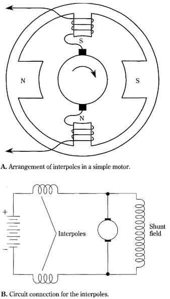
FIG. 6 The use of interpoles for improving commutation.

A. Arrangement of interpoles in a simple motor. Shunt field

B. Circuit connection for the interpoles.

Additional techniques for improving commutation

Frequently, dc machines are encountered in which the brush axis is in the geometrical plane and neither compensating windings nor interpoles are utilized. However, there might be more than meets the eye in the design of the machine. For example, FIG. 7 illustrates three techniques that can be quite effective in negating the com mutation-degrading effects of armature reaction, self-inductance, and mutual inductance associated with the armature conductors.

FIG. 7A depicts an armature loop being shorted by a brush bearing on the two commutator segments to which the ends of the loop are connected. The brush is processed so that its resistivity is reasonably low in the brush plane that accommodates current to, or from, the armature. In the illustration this is the vertical plane. But, the resistivity crosswise through the brush is relatively high—that is, in the horizontal plane along which the short circuit current must flow, high resistivity is encountered.

The scheme shown in FIG. 7B uses a pole structure shaped so that the magnetic reluctance in the regions of the pole tips is greatly increased. This can be brought about by the use of a nonconcentric curvature of the pole face so that the radial distance between the armature and the pole face is greater near the tips than in the central region. In the illustration, field flux is shown but no current is flowing in the armature conductors. Notice that the field density is relatively sparse in the regions of the pole tips. This condition is opposite to that occurring with conventionally shaped field poles and with armature current flowing. Therefore, the “pinched” field configuration shown to produce when current is flowing in the armature.

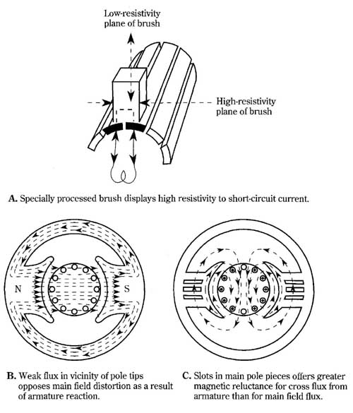
FIG. 7 Additional techniques for improving commutation.

A. Specially processed brush displays high resistivity to short-circuit current. Low-resistivity plane of brush; High-resistivity plane of brush

B. Weak flux in vicinity of pole tips opposes main field distortion as a result of armature reaction.

C. Slots in main pole pieces offers greater magnetic reluctance for cross flux from armature than for main field flux.

A somewhat more sophisticated method of combating armature reaction is shown in FIG. 7C. Here, the pole piece is slotted to offer high magnetic reluctance to the cross field associated with the current-carrying armature. The armature flux, therefore, has diminished strength with which to distort the main field. In this example, it is expedient to show the armature flux instead of the main field flux.

Machine function and reversal of rotation

Because of the counter EMF generated in dc motors, and the countertorque produced in dc generators, a machine that ordinarily performs the function of a motor be comes a generator by interchanging the forms of energy supplied and extracted. The reverse interchange converts a machine normally used as a generator into a motor.

The reciprocal functions of these dc machines are not always so simply implemented. For example, the brushes of a motor can be positioned at some angular distance from geometric neutral in order to obtain good commutation. If the machine is pressed into service as a generator, severe sparking is likely to occur. For the same armature current in a machine used as a generator, the proper brush position is now approximately the same angular distance on the other side of the geometric neutral axis. Also, brushes that have other than a radial orientation with respect to the commutator do not always provide satisfactory electrical or mechanical performance when the rotation of the armature is reversed.

A common trouble encountered in reversing motors stems from ignoring the series field in compound motors. If, for example, such a motor is reversed by transposing the connections to the armature alone, the operating characteristics will be changed from those of a cumulative compound motor to those of a differential com pound motor, or vice-versa. The same logic applies to the compound dc generator when the polarity is changed in the same manner. In both compound motors and generators, the leads common to the armature and the series field must not be disconnected. The two remaining leads are then transposed in order to reverse rotation in the motor, or reverse polarity in the generator.

The same reasoning also applies to compensating windings and to interpoles. However, the situation is less likely to involve trouble or confusion with such connections because they are usually not as accessible. For example, one armature lead of a shunt motor with interpoles will actually be the commutator brush. The other “armature” lead, however, will usually be one end of the interpole coils. (The other end of the interpole coils is permanently corrected to the opposite brush.) Whether the machine functions as a motor or as a generator, and regardless of its rotation, such poles or windings will always be properly connected.

The simplest case of all pertains to having no interpoles, compensating windings, or compounding windings, and in which the brush axis coincides with geometric neutral. With such machines, equally acceptable commutation can be obtained regardless of direction or function.

Speed behavior of dc shunt motors

The speed control characteristics of the dc shunt motor are particularly important because they are often the basis for comparison with other types of motors. Of special interest is the speed behavior with respect to variable field current. Does greater field strength make the speed increase or decrease? This is hardly a trivial question; unless you are already knowledgeable in this matter, it’s easy to get confused. For example, the three control situations depicted in FIG. 8 all achieve speed variation by controlling the field current. Yet, the individual behavior of each appears to contradict rather than confirm any basic rule. The “shunt motor” shown in FIG. 8A is actually a dc watt-hour meter. The more current passed through its field, the greater the speed developed by this small machine. The conventional shunt motor shown in FIG. 8B behaves in opposite fashion; the greater the field current, the slower the speed. Finally, the motor of FIG. 8C is again a shunt motor, although it might bear the specialized nomenclature of “servo motor.” Here, as with the dc watt-hour meter, increased field current results in higher speed.

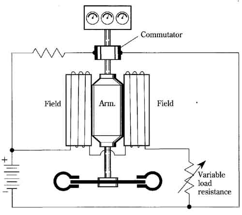
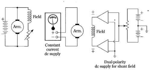
FIG. 8 Field control of dc shunt motors.

A. A dc watt-hour meter. B. A conventional dc shunt motor. Constant current dc supply; C. A servo motor. The field is operated from an amplifier arrangement that allows for polarity reversal in order that the motor can be run in either direction. Dual-polarity dc supply for shunt field

In order to gain insight into these apparent inconsistencies, try to reconcile two equations, both of which are valid but appear to suggest divergent interpretations. The generalized formula for the torque, T, of any dc motor can be stated as follows:

T = k PHI I_a

where:

k represents the number of poles, armature paths, and conductors,

PHI is the flux per pole that links the armature conductors, and I_a is the armature current.

Don’t be concerned with units; rather, try to pin down the qualitative reasons for the divergent speed characteristics described on previous page. Use these equations to facilitate this objective, rather than to provide the background for numerical solutions. The second equation, which gives the speed of dc motors, is stated as follows:

s = V_a — (I_a x R_a)/k PHI

where,

V_a is the voltage across the armature terminals,

I_a is the armature current,

R_a is the armature resistance,

k is the number of poles, armature paths, and conductors, and

PHI is the flux per pole that links the armature conductors.

The first equation leads you to believe that a stronger field should result in greater speed. Although speed is not a parameter of the first equation, the torque is a “prime mover” of speed. Surely, if more torque is developed in an operating motor, the torque must, among other things, manifest itself as acceleration of the rotating armature. The second equation apparently contradicts such an interpretation. Be cause the quantity PHI now appears in the denominator, you might expect an increase in field strength to produce a decrease in speed.

Unfortunately, neither of these equations reveals an important characteristic of dc shunt machines. The armature current and field flux in both equations are not in dependent quantities. The numerator of the second equation is actually the counter EMF and can significantly affect armature current—a torque-producing factor. The counter EMF, in turn, is governed by PHI.

In conventional motors, a small change in field strength produces a much greater percentage of change in armature current. For example, if PHI is increased in the first equation, ‘a will be reduced to the extent that the torque will actually de crease. Because of this, you must anticipate a decrease in speed. However, some care is needed in order to confirm this when you are dealing with the second equation. What neither equation tells us is that dc motors (and generators) are actually power amplifiers. In these machines, a small change in the power applied to the field is manifested by a large change in the power consumed (motor) or delivered (generator) by the armature. The change in armature power level is primarily caused by the variation in armature current.

Now justify the speed characteristics displayed in the three shunt motor situations of FIG. 8. The “air-core” shunt motor, or watt-hour meter of FIG. 8A, does not generate much counter EMF; that is, the counter EMF is low compared with voltage T impressed across the armature. Unlike the situation prevailing in conventional machines, the counter EMF is not a strong function of field strength t. Therefore, when PHI is increased, the first equation, T = k PHI I_a tells us that the torque, T, will also become greater. This being the case, you would expect the armature to accelerate toward a higher speed. Can this be confirmed with the second equation:

S = V_a – (I_a R_a) / k PHI

For the qualitative purpose involved, inject some numbers that can be handled with easy mental arithmetic. Let T = 100 volts. And, because we know that the counter EMF is low, the armature-resistance voltage drop, IaRa will be very close to 99 volts. Finally, assume that the product of k and 1 is 0.10 and that this enables the speed, S, to be expressed in revolutions per minute. Making the appropriate substitutions, we have:

S = 100-99/0.10 = 10 RPM

Let the field strength be increased by 10 percent, and assume that this leads to a decrease in armature current of approximately one percent. You are guided in making such an assumption by the known generator action of this device—that is, by the low counter EMF produced. Otherwise, the quantitative significance of our numbers is of no great importance for our goal, which is to ascertain which way the speed changes with respect to field strength. Again, making the appropriate substitutions, we now have:

s = 10 = 10 RPM

Thus, the speed has increased with increasing field strength. (Inasmuch as the interest here is not in the instrumental aspects of the basic shunt motor used in the dc watt-hour meter, the action of the shaft-attached, eddy-current disk has not been mentioned. However, its function is to impose a countertorque directly proportional to speed. This brings about the desirable operating feature of the speed of the over all device becoming proportional to the power supplied to the load.) With the discussion of this device as a prelude, a similar investigation for the conventional shunt motor of FIG. 8B is now conducted.

Because the conventional shunt motor has iron in its magnetic circuit, the counter EMF will tend to be close to the voltage applied across the armature terminals. However, the voltage drop across the armature will tend to remain relatively small. These facts will always hold true for a shunt motor that is operating at a constant speed with a fixed load within its ratings. Obviously, under such conditions, the motor must be simultaneously operating as a generator that produces a voltage in opposition to the impressed armature voltage. Only a small portion of the impressed voltage is actually available to force current through the armature resistance in accordance with Ohm’s law. Assuming such a motor is operating with a moderate load at a constant speed, what happens to the speed when the field current, and there fore the field strength, is increased?

A casual inspection of the speed equation,

S = V_a – (I_a R_a) / k PHI

certainly suggests a reduction in speed. The impressed armature voltage, V_a is fixed; k is a constant associated with the particular machine; and there is no change in the armature resistance, Ra It would appear that the armature current, ‘a’ would have to adjust itself to the new conditions, but you have to know in which direction this change in armature current will occur and the relative magnitude of the change. Otherwise, you might be led to an erroneous interpretation when attempting to reconcile the torque equation with the speed equation. The torque equation, T = k 1 ‘a’ seemingly suggests that, on the basis of field strength I alone, torque T increases. This would imply that the motor accelerates when is made greater, which would lead to higher speed. The fact that the motor actually slows down when its field cur rent (field strength) is increased imposes a dilemma.

The resolution of this paradoxical situation requires insight beyond that pro vided by the mere mathematical interpretations of the two equations. Actually, when PHI is increased, the resultant increase in counter EMF developed in the armature reduces the armature current taken from the dc source. The reduction in armature current I_a is, by virtue of the “amplifying action” of the machine, proportionally greater than the increase in field strength t. Therefore, the apparently strange fact that torque T is reduced must be accepted. Reduced torque must manifest itself in a slowing down of the motor!

The slowed motor then develops a lower counter EMF. This, in turn, allows more armature current. Ultimately, the motor is operating at a slower speed but has reestablished equilibrium with the same counter EMF and the same armature cur rent as prevailed before the field was increased.

The speed of shunt motors is ordinarily controlled over a range of field current, and the field strength, PHI, is directly proportional to the field current. Outside of this range, there is either diminishing returns from the effect of magnetic saturation of the iron in the pole structure or operational instability and poor commutation be cause of armature reaction.

In practice, the speed equation is not used in an absolute sense. That is, it is not generally used for predicting motor speed “from scratch.” Rather, it is used to set up a proportion from previously measured parameters obtained from an operating motor. Thus, you might have recorded T ‘a’ Ra the field current and the speed. If the field current is increased by ten percent, it is easy enough to deduce that the speed will be decreased by ten percent.

The motor depicted in FIG. 8C could be the same one just discussed in the simpler control arrangement shown in FIG. 8B. However, the speed behavior is altogether different—now the motor speeds up in response to higher field current. A more complex field current supply and a separate power source for the armature is shown.

The singular item responsible for this perhaps unexpected speed characteristic is the constant current supply for the armature. It is the basic nature of a constant current source that the voltage delivered to a variable load varies widely. It is this varying voltage that enables the current delivered to the load to be maintained constant. This is one of two important factors in this speed-control technique. The other factor is the influence of the applied armature voltage, V_a, in the speed equation:

S = V_a – (I_a R_a) / k PHI

A little more consideration will show that the speed would be almost directly proportional to T if it alone were varied and if all other parameters remained constant. Although no voltage-control technique is shown associated with the motor armature, the use of the constant current supply varies the voltage applied to the armature. From previous discussions, you know that a small increase in field strength produces a large reduction in armature current. Inasmuch as the armature current change would have been great with respect to the change in field strength, the constant cur rent source is forced to make a large change in armature voltage in order to maintain the armature current constant. Therefore, armature voltage becomes the governing factor in the speed equation. Its position in the speed equation enables it to influence speed very nearly on a directly proportional basis—that is, S tends to be proportional to Ea. (Actually, the field-current supply need be nothing more involved than a battery and a rheostat. The arrangement illustrated is suggestive of a servo-amplifier application in which the motor can be operated in either direction.)

Before applying electronic controls to motors and generators, it is necessary to be familiar with the “natural” performance of these machines. In general, two methods of plotting motor characteristics assume importance, although additional plot ting techniques are used occasionally. In one of the main methods, the various operating parameters of a motor are plotted as functions of armature current. Thus, you might be interested in speed versus armature current, or torque versus armature current. For these purposes, armature current is plotted on the horizontal axis because it is considered the independent variable.

This way of looking at motor performance is primarily of interest to the engineer, the student, or anybody who wants to gain insight into the basic operating mechanism of the motor. The user is not greatly concerned with armature current once the basic requisites of wire size, fuse or circuit-breaker capacity, and power source are taken care of. (Sometimes the armature-current quantity in a shunt motor might also include the field current. In such a case, it is erroneous to consider the total line current the same as the armature current alone. But, because the shunt motor field current tends to be a small percentage of armature current, especially when the motor is appreciably loaded, the error of such a presentation is often not of great consequence. In series motors and permanent-magnet motors, armature current and line current are identical.)

The user is more interested in the usable quantity available from the shaft— this quantity is the turning power, or torque, of the motor. That is why graphs of mo tor performance often depict speed, horsepower, efficiency, etc., as functions of a torque, rather than of armature current.

As mentioned before, other graphical formats are also used. For example, the user might be interested in the quantity of horsepower rather than torque that is de livered by the motor shaft. Horsepower comprises the two factors of speed and torque. Torque, on the other hand, does not involve speed. Indeed, one of the important things revealed by a graph plotted against torque is the turning power of the motor at zero speed—this is the starting torque.

Often, the same information can be revealed by different plotting methods, and the choice is then determined by convenience of interpretation. If you were considering some kind of a control for an automotive starter motor, for example, you certainly would be interested in seeing a graph depicting speed versus torque. But, you would also like to see torque plotted as a function of armature current. Graphs with specialized formats to emphasize the behavior of efficiency or horsepower could conceivably prove useful too. From the standpoint of control, plots of motor characteristics versus field current can be of prime importance when dealing with shunt- field and compound-field machines.

Basic characteristics of the shunt motor

The speed and torque characteristic of a dc shunt motor are shown in FIG. 9. Loosely speaking, the shunt motor can be called a constant-speed machine. Indeed, the effects of armature reaction and magnetic saturation often tend to make the speed curve even flatter than that illustrated in the graph of FIG. 9B. At first, it might seem that the performance curves of shunt motors reveal the operation of permanent-magnet motors also. However, there can be significant differences in the region of overload. Instead of the speed encountering a “breakdown” region, such as is depicted by the dashed portion of the curve in FIG. 9B, a permanent-magnet mo tor can have a linearly sloped speed characteristic right down to zero speed. This implies greater torque at low speeds. Because a motor is at zero speed just prior to starting, the permanent-magnet motor is capable of exerting higher starting torque than its equivalently rated shunt machine (in terms of horsepower).

The above described differences are largely brought about by the different conditions of armature reaction of the two types of motors. However, much depends on the selection of magnet materials and on other design factors. It does not necessarily follow that the permanent-magnet motor will feature this extraordinary behavior. Older designs often gave poor accounts of themselves in actual service because of susceptibility to demagnetization from the effects of armature reaction. Because of advanced materials technology, and sometimes because of the inclusion of compensating windings in the pole faces, this shortcoming has largely been overcome.

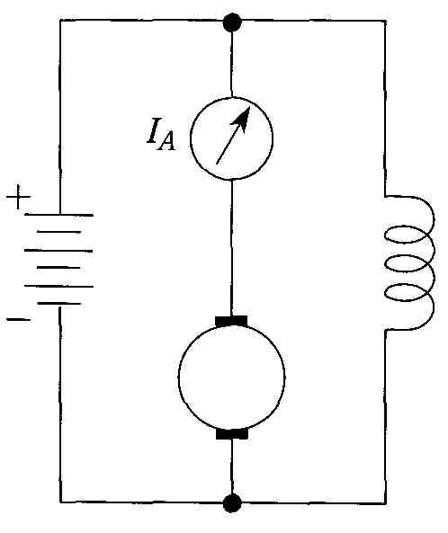
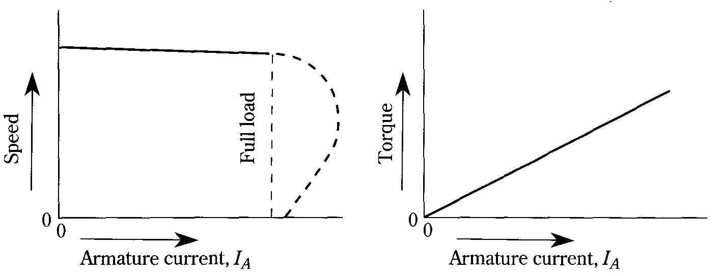
FIG. 9 Speed and torque of a shunt motor as a function of armature current. A. Shunt motor circuit. B. Speed versus armature current. C. Torque versus armature current.

In FIG. 10, the speed versus armature current behavior of the shunt motor is extended for the situation in which resistance is inserted in the armature circuit (Ra) and in the field circuit(Ra). The actual variation in armature current is intentionally caused by varying the mechanical load applied to the shaft. Significantly, the use of armature resistance enables lower speed ranges to be attained. In contrast, when resistance is inserted in the field circuit, higher speed ranges become available. A shortcoming of the use of armature resistance is that it deprives the motor of its near-constant speed behavior. Also, the power dissipation in this resistance presents serious problems in larger motors. From casual inspection of the graph in FIG. bC, the field-resistance method of speed control displays no disadvantageous features (other than the inability to acquire lower speed ranges). However, the weakening of the field increases its vulnerability to distortion from armature reaction. Attempts to reduce speed by a factor exceeding about four to one by this method tend to cause commutation difficulties and operating instability.

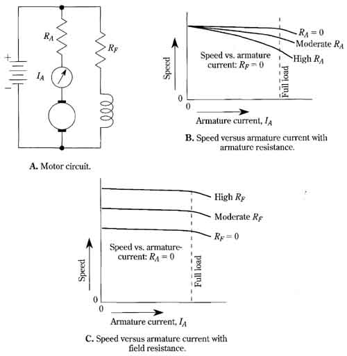
FIG. 10 Speed behavior of the shunt motor with armature or field resistance. A. Motor circuit. B. Speed versus armature current with armature resistance. C. Speed versus armature current with field resistance.

Motor speed control by shunt field current

FIG. 11 illustrates the general situation prevailing in dc shunt motors when the speed is controlled by the field current. Interestingly, the control could be usefully extended to a speed range well below the rated speed if it were not for the magnetic saturation of the field iron. With actual machines, the control region above the rated field current is in an area of diminishing returns even if you are interested in only limited-duration applications of high field current.

If the field current is reduced in order to operate the motor at a higher speed, the armature current corresponding to the higher speed operation is substantially the same as it was for the slower speed. The assumption is made that the torque demand of the load remains constant. Nonetheless, when the field current in a shunt motor is reduced during operation, dangerously high armature current might result, particularly in large machines.

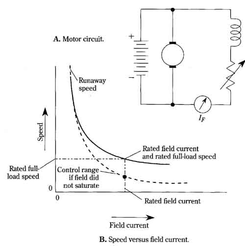
FIG. 11 Speed as a function of field current in a shunt motor. A. Motor circuit. B. Speed versus field current.

The apparent contradiction in the above paragraph is resolved as follows: When the field current is first reduced, the counter EMF almost immediately follows suit. This causes a large inrush of armature current. The resultant accelerating torque will ultimately develop a high enough speed that the counter EMF will admit only enough cur rent to accommodate the torque demand of the load. But, because of the rotational inertia of the armature, and often of the load, this corrective action cannot take place instantly. Thus, while the motor is accelerating, very high armature currents can exist.

The action described above becomes dangerous at low field currents, and particularly at zero field current. This is the “runaway” region depicted by the dotted portion of the speed curve in FIG. 11. The action is not qualitatively different from that described for the normal range of control by field-current variation. However, the motor now seeks a fantastically high speed to restore its operating equilibrium. Before this speed can even be approached, the armature might explode from centrifugal forces or the motor might suffer damage from the tremendous current in rush. The tendency is similar whether or not the motor is loaded; when loaded, the self-destruction by racing might take a little longer, but the damage caused by excessive current is likely to occur more quickly.

Non-rheostat control of armature voltage

Before the development of solid-state devices, specifically the power transistor and the thyristor, armature-voltage control of shunt motors was accomplished by means of rheostats or tapped resistors. The high-power dissipation involved imposed practical difficulties in implementation and would have been economically devastating in the long run, due to the waste of electrical energy. Also, the resistance in the armature cir cult resulted in poorer speed regulation. It was found that, except for initial cost, the above disadvantages could be largely overcome by powering the armature of the con trolled motor from the output of a generator, which in turn could have its output con trolled by its own field current. The motor then would “see” a variable-voltage power source—one in which the internal resistance was always very low. A motor controlled in this manner responded by displaying excellent starting characteristics, minimal com mutation difficulties, and an inordinately wide range of speed control. This control technique, known as the Ward-Leonard system, is shown in FIG. 12.

In FIG. 13A, the characteristics of an armature-voltage controlled motor are shown. The variable-voltage power supply can be a regulated power supply with low output impedance. More often, however, it is a thyristor circuit in which the aver age output voltage is varied by phase control of the firing angle. Pulse-width-modulated switching transistors can be employed in a similar manner. Such a control method can be electrically efficient and quite economical compared with older control methods. This is especially true with large machines, in which case the thyristor presently predominates. Moreover, such armature-voltage control is applicable in the same way to permanent-magnet motors.

The control method illustrated in FIG. 13B is similar, except that both armature and field voltages are controlled together. The speed and torque curves then have the general shapes shown. Starting torque is appreciably lower in this arrangement than in that of FIG. 13A. However, a separate field supply is not needed.

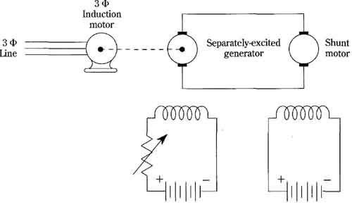
FIG. 12 The Ward-Leonard speed control system for dc shunt motors. 3 PHI Line, 3 PHI Induction motor, Shunt motor

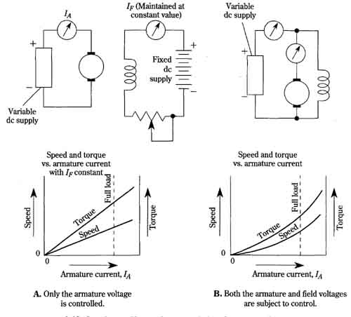
FIG. 13 Speed control by non-rheostat variation of armature voltage. A. Only the armature voltage is controlled. B. Both the armature and field voltages are subject to control. I_F (Maintained at constant value); Variable dc supply; Speed and torque vs. armature current with I_F constant

In the control circuits of FIG. 13, the fully rated mechanical load is already coupled to the motor shaft. Then, the armature voltage is brought up from zero, with the speed and torque parameters being recorded with respect to increments of armature current.