AMAZON multi-meters discounts AMAZON oscilloscope discounts
Voltage sags are short duration reductions in rms voltage, mainly caused by short circuits and starting of large motors. The interest in voltage sags is due to the problems they cause on several types of equipment.
Adjustable-speed drives, process-control equipment, and computers are especially notorious for their sensitivity. Some pieces of equipment trip when the rms voltage drops below 90% for longer than one or two cycles. Such a piece of equipment will trip tens of times a year. If this is the process-control equipment of a paper mill, one can imagine that the costs due to voltage sags can be enormous. A voltage sag is not as damaging to industry as a (long or short) interruption, but as there are far more voltage sags than interruptions, the total damage due to sags is still larger. Another important aspect of voltage sags is that they are hard to mitigate. Short interruptions and many long interruptions can be prevented via simple, although expensive measures in the local distribution network. Voltage sags at equipment terminals can be due to short-circuit faults hundreds of kilo meters away in the transmission system. It will be clear that there is no simple method to prevent them.
1. Voltage Sag Characteristics
An example of a voltage sag is shown in FIG. 1. The voltage amplitude drops to a value of about 20% of its pre-event value for about two and a half cycles, after which the voltage recovers again. The event shown in FIG. 1 can be characterized as a voltage sag down to 20% (of the pre-event voltage) for 2.5 cycles (of the fundamental frequency). This event can be characterized as a voltage sag with a magnitude of 20% and a duration of 2.5 cycles.
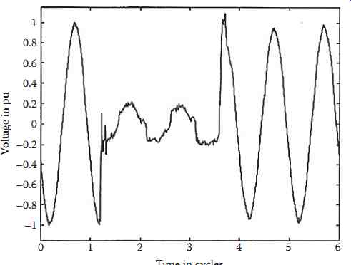
FIG. 1 A voltage sag-voltage in one phase in time domain.
1.1 Voltage Sag Magnitude: Monitoring
The magnitude of a voltage sag is determined from the rms voltage. The rms voltage for the sag in FIG. 1 is shown in FIG. 2. The rms voltage has been calculated over a one-cycle sliding window:
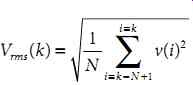
(eqn 1)
with N the number of samples per cycle, and v(i) the sampled voltage in time domain. The rms voltage as shown in FIG. 2 does not immediately drop to a lower value, but takes one cycle for the transition. This is due to the finite length of the window used to calculate the rms value. We also see that the rms value during the sag is not completely constant and that the voltage does not immediately recover after the fault.
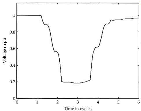
FIG. 2 One-cycle rms voltage for the voltage sag shown in FIG. 1.
There are various ways of obtaining the sag magnitude from the rms voltages. Most power quality monitors take the lowest value obtained during the event. As sags normally have a constant rms value during the deep part of the sag, using the lowest value is an acceptable approximation.
The sag is characterized through the remaining voltage during the event. This is then given as a percentage of the nominal voltage. Thus, a 70% sag in a 230-V system means that the voltage dropped to 161 V. The confusion with this terminology is clear. One could be tricked into thinking that a 70% sag refers to a drop of 70%, thus a remaining voltage of 30%. The recommendation is therefore to use the phrase "a sag down to 70%." Characterizing the sag through the actual drop in rms voltage can solve this ambiguity, but this will introduce new ambiguities like the choice of the reference voltage.
1.2 Origin of Voltage Sags
Consider the distribution network shown in FIG. 3, where the numbers (1 through 5) indicate fault positions and the letters (A through D) loads. A fault in the transmission network, fault position 1, will cause a serious sag for both substations bordering the faulted line. This sag is transferred down to all customers fed from these two substations. As there is normally no generation connected at lower voltage levels, there is nothing to keep up the voltage. The result is that all customers (A, B, C, and D) experience a deep sag. The sag experienced by A is likely to be somewhat less deep, as the generators connected to that substation will keep up the voltage. A fault at position 2 will not cause much voltage drop for customer A. The impedance of the transformers between the transmission and the subtransmission system are large enough to considerably limit the voltage drop at high-voltage side of the transformer. The sag experienced by customer A is further mitigated by the generators feeding into its local transmission substation. The fault at position 2 will, however, cause a deep sag at both subtransmission substations and thus for all customers fed from here (B, C, and D). A fault at position 3 will cause a short or long interruption for customer D when the protection clears the fault. Customer C will only experience a deep sag. Customer B will experience a shallow sag due to the fault at position 3, again due to the transformer impedance. Customer A will probably not notice anything from this fault. Fault 4 causes a deep sag for customer C and a shallow one for customer D. For fault 5, the result is the other way around: a deep sag for customer D and a shallow one for customer C. Customers A and B will not experience any significant drop in voltage due to faults 4 and 5.
FIG. 3 Distribution network with load positions (A through D) and fault positions
(1 through 5).
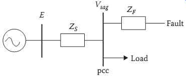
FIG. 4 Voltage divider model for a voltage sag.
1.3 Voltage Sag Magnitude: Calculation
To quantify sag magnitude in radial systems, the voltage divider model, shown in FIG. 4, can be used, where Z is the source impedance at the point-of-common coupling; and Z is the impedance between the point-of-common coupling and the fault. The point-of-common coupling (pcc) is the point from which both the fault and the load are fed. In other words, it is the place where the load current branches off from the fault current. In the voltage divider model, the load current before, as well as during the fault is neglected. The voltage at the pcc is found from
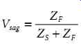
(eqn 2)
where it is assumed that the pre-event voltage is exactly 1 pu, thus E = 1. The same expression can be derived for constant-impedance load, where E is the pre-event voltage at the pcc. We see from Equation 2 that the sag becomes deeper for faults electrically closer to the customer (when ZF becomes smaller), and for weaker systems (when ZS becomes larger).
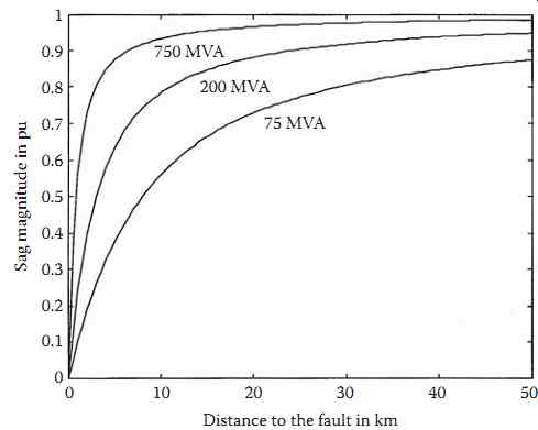
FIG. 5 Sag magnitude as a function of the distance to the fault.
Equation 2 can be used to calculate the sag magnitude as a function of the distance to the fault.
Therefore, we write ZF = zd, with z the impedance of the feeder per unit length and d the distance between the fault and the pcc, leading to
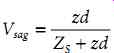
(eqn 3)
This expression has been used to calculate the sag magnitude as a function of the distance to the fault for a typical 11 kV overhead line, resulting in FIG. 5. For the calculations, a 150-mm2 overhead line was used and fault levels of 750, 200, and 75 MVA. The fault level is used to calculate the source impedance at the pcc and the feeder impedance is used to calculate the impedance between the pcc and the fault. It is assumed that the source impedance is purely reactive, thus ZS = j 0.161 ohm for the 750 MVA source. The impedance of the 150 mm2 overhead line is z = 0.117 + j 0.315 ohm/km.
1.4 Propagation of Voltage Sags
It is also possible to calculate the sag magnitude directly from fault levels at the pcc and at the fault position. Let SFLT be the fault level at the fault position and SPCC at the point-of-common coupling. The voltage at the pcc can be written as
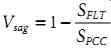
(eqn 4)
This equation can be used to calculate the magnitude of sags due to faults at voltage levels other than the point-of-common coupling. Consider typical fault levels as shown in Table 1. This data has been used to obtain Table 2, showing the effect of a short circuit fault at a lower voltage level than the pcc.
We can see that sags are significantly "damped" when they propagate upwards in the power system. In a sags study, we typically only have to take faults one voltage level down from the pcc into account. And even those are seldom of serious concern. Note, however, that faults at a lower voltage level may be associated with a longer fault-clearing time and thus a longer sag duration. This especially holds for faults on distribution feeders, where fault-clearing times in excess of 1 s are possible.
1.5 Critical Distance
Equation 3 gives the voltage as a function of distance to the fault. From this equation we can obtain the distance at which a fault will lead to a sag of a certain magnitude V. If we assume equal X/R ratio of source and feeder, we get the following equation:
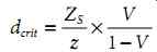
(eqn 5)
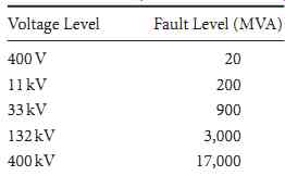
TABLE 1 Typical Fault Levels at Different Voltage Levels
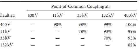
TABLE 2 Propagation of Voltage Sags to Higher Voltage Levels
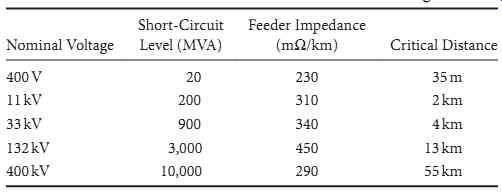
TABLE 3 Critical Distance for Faults at Different Voltage Levels
We refer to this distance as the critical distance. Suppose that a piece of equipment trips when the volt age drops below a certain level (the critical voltage). The definition of critical distance is such that each fault within the critical distance will cause the equipment to trip. This concept can be used to estimate the expected number of equipment trips due to voltage sags. The critical distance has been calculated for different voltage levels, using typical fault levels and feeder impedances. The data used and the results obtained are summarized in Table 3 for the critical voltage of 50%. Note how the critical distance increases for higher voltage levels. A customer will be exposed to much more kilometers of transmission lines than of distribution feeder. This effect is understood by writing Equation 5 as a function of the short-circuit current Iflt at the pcc:
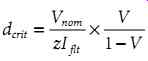
(eqn 6)
with Vnom the nominal voltage. As both z and Iflt are of similar magnitude for different voltage levels, one can conclude from Equation 6 that the critical distance increases proportionally with the voltage level.
1.6 Voltage Sag Duration
It was shown before, the drop in voltage during a sag is due to a short circuit being present in the system.
The moment the short circuit fault is cleared by the protection, the voltage starts to return to its original value. The duration of a sag is thus determined by the fault-clearing time. However, the actual duration of a sag is normally longer than the fault-clearing time.
Measurement of sag duration is less trivial than it might appear. From a recording the sag duration may be obvious, but to come up with an automatic way for a power quality monitor to obtain the sag duration is no longer straightforward. The commonly used definition of sag duration is the number of cycles during which the rms voltage is below a given threshold. This threshold will be somewhat different for each monitor but typical values are around 90% of the nominal voltage. A power quality monitor will typically calculate the rms value once every cycle.
The main problem is that the so-called post-fault sag will affect the sag duration. When the fault is cleared, the voltage does not recover immediately. This is mainly due to the reenergizing and reacceleration of induction motor load. This post-fault sag can last several seconds, much longer than the actual sag. Therefore, the sag duration as defined before, is no longer equal to the fault clearing time. More seriously, different power quality monitors will give different values for the sag duration. As the rms voltage recovers slowly, a small difference in threshold setting may already lead to a serious difference in recorded sag duration.
Generally speaking, faults in transmission systems are cleared faster than faults in distribution systems. In transmission systems, the critical fault-clearing time is rather small. Thus, fast protection and fast circuit breakers are essential. Also, transmission and subtransmission systems are normally operated as a grid, requiring distance protection or differential protection, both of which allow for fast clearing of the fault. The principal form of protection in distribution systems is overcurrent protection. This requires a certain amount of time-grading, which increases the fault-clearing time. An exception is formed by systems in which current-limiting fuses are used. These have the ability to clear a fault within one half-cycle. In overhead distribution systems, the instantaneous trip of the recloser will lead to a short sag duration, but the clearing of a permanent fault will give a sag of much longer duration.
The so-called magnitude-duration plot is a common tool used to show the quality of supply at a certain location or the average quality of supply of a number of locations. Voltage sags due to faults can be shown in such a plot, as well as sags due to motor starting, and even long and short interruptions. Different underlying causes lead to events in different parts of the magnitude-duration plot, as shown in FIG. 6.
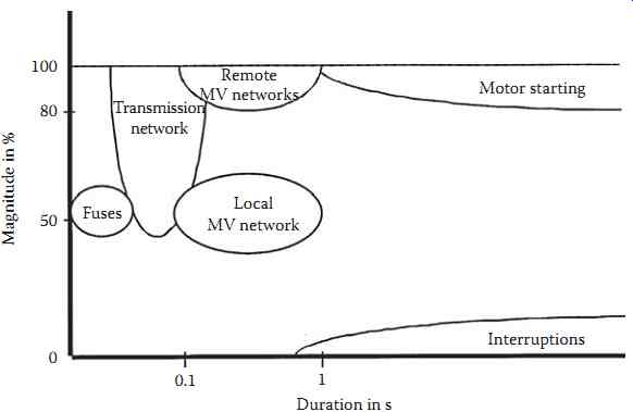
FIG. 6 Sags of different origin in a magnitude-duration plot.
1.7 Phase-Angle Jumps
A short circuit in a power system not only causes a drop in voltage magnitude, but also a change in the phase angle of the voltage. This sudden change in phase angle is called a "phase-angle jump." The phase-angle jump is visible in a time-domain plot of the sag as a shift in voltage zero-crossing between the pre-event and the during-event voltage. With reference to FIG. 4 and Equation 2, the phase angle jump is the argument of Vsag, thus the difference in argument between ZF and ZS + ZF. If source and feeder impedance have equal X/R ratio, there will be no phase-angle jump in the voltage at the pcc.
This is the case for faults in transmission systems, but normally not for faults in distribution systems.
The latter may have phase-angle jumps up to a few tens of degrees.
FIG. 4 shows a single-phase circuit, which is a valid model for three-phase faults in a three-phase system. For nonsymmetrical faults, the analysis becomes much more complicated. A consequence of nonsymmetrical faults (single-phase, phase-to-phase, two-phase-to-ground) is that single-phase load experiences a phase-angle jump even for equal X/R ratio of feeder and source impedance.
To obtain the phase-angle jump from the measured voltage waveshape, the phase angle of the voltage during the event must be compared with the phase angle of the voltage before the event. The phase angle of the voltage can be obtained from the voltage zero-crossings or from the argument of the fundamental component of the voltage. The fundamental component can be obtained by using a discrete Fourier trans form algorithm. Let V1(t) be the fundamental component obtained from a window (t-T,t), with T one cycle of the power frequency, and let t = 0 correspond to the moment of sag initiation. In case there is no chance in voltage magnitude or phase angle, the fundamental component as a function of time is found from
(eqn. 7)
The phase-angle jump, as a function of time, is the difference in phase angle between the actual fundamental component and the "synchronous voltage" according to Equation 7:
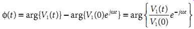
(eqn 8)
Note that the argument of the latter expression is always between -180° and +180°.
1.8 Three-Phase Unbalance
For three-phase equipment, three voltages need to be considered when analyzing a voltage sag event at the equipment terminals. For this, a characterization of three-phase unbalanced voltage sags is introduced. The basis of this characterization is the theory of symmetrical components. Instead of the three phase voltages or the three symmetrical components, the following three (complex) values are used to characterize the voltage sag:
• The "characteristic voltage" is the main characteristic of the event. It indicates the severity of the sag, and can be treated in the same way as the remaining voltage for a sag experienced by a single phase event.
• The "PN factor" is a correction factor for the effect of the load on the voltages during the event.
The PN factor is normally close to unity and can then be neglected. Exceptions are systems with a large amount of dynamic load, and sags due to two-phase-to-ground faults.
• The "zero-sequence voltage," which is normally not transferred to the equipment terminals, rarely affects equipment behavior. The zero-sequence voltage can be neglected in most studies.
Neglecting the zero-sequence voltage, it can be shown that there are two types of three-phase unbalanced sags, denoted as types C and D. Type A is a balanced sag due to a three-phase fault. Type B is the sag due to a single-phase fault, which turns into type D after removal of the zero-sequence voltage. The three complex voltages for a type C sag are written as follows:
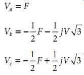
(eqn 9)
...where V is the characteristic voltage and F the PN factor. The (characteristic) sag magnitude is defined as the absolute value of the characteristic voltage; the (characteristic) phase-angle jump is the argument of the characteristic voltage. For a sag of type D, the expressions for the three voltage phasors are as follows:
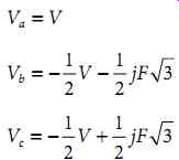
(eqn 10)
Sag type D is due to a phase-to-phase fault, or due to a single-phase fault behind a [delta]y-transformer, or a phase-to-phase fault behind two [delta]y-transformers, etc. Sag type C is due to a single-phase fault, or due to a phase-to-phase fault behind a [delta]y-transformer, etc. When using characteristic voltage for a three phase unbalanced sag, the same single-phase scheme as in FIG. 4 can be used to study the transfer of voltage sags in the system.
2. Equipment Voltage Tolerance
2.1 Voltage Tolerance Requirement
Generally speaking, electrical equipment prefers a constant rms voltage. That is what the equipment has been designed for and that is where it will operate best. The other extreme is zero voltage for a longer period of time. In that case the equipment will simply stop operating completely. For each piece of equipment there is a maximum interruption duration, after which it will continue to operate correctly. A rather simple test will give this duration. The same test can be done for a voltage of 10% (of nominal), for a voltage of 20%, etc. If the voltage becomes high enough, the equipment will be able to operate on it indefinitely. Connecting the points obtained by performing these tests results in the so-called "voltage-tolerance curve". An example of a voltage-tolerance curve is shown in FIG. 7: the requirements for IT-equipment as recommended by the Information Technology Industry Council (ITIC). Strictly speaking, one can claim that this is not a voltage-tolerance curve as described above, but a requirement for the voltage tolerance. One could refer to this as a voltage-tolerance requirement and to the result of equipment tests as a voltage-tolerance performance.
We see in FIG. 7 that IT equipment has to withstand a voltage sag down to zero for 1.1 cycle, down to 70% for 30 cycles, and that the equipment should be able to operate normally for any voltage of 90% or higher.
2.2 Voltage Tolerance Performance
Voltage-tolerance (performance) curves for personal computers are shown in FIG. 8. The curves are the result of equipment tests performed in the United States and in Japan. The shape of all the curves in FIG. 8 is close to rectangular. This is typical for many types of equipment, so that the voltage tolerance may be given by only two values, maximum duration and minimum voltage, instead of by a full curve. From the tests summarized in FIG. 8 it is found that the voltage tolerance of personal computers varies over a wide range: 30-170 ms, 50%-70% being the range containing half of the models. The extreme values found are 8 ms, 88% and 210 ms, 30%.
Voltage-tolerance tests have also been performed on process-control equipment: PLCs, monitoring relays, motor contactors. This equipment is even more sensitive to voltage sags than personal computers. The majority of devices tested tripped between one and three cycles. A small minority was able to tolerate sags up to 15 cycles in duration. The minimum voltage varies over a wider range: from 50% to 80% for most devices, with exceptions of 20% and 30%. Unfortunately, the latter two both tripped in three cycles.
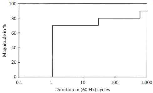
FIG. 7 Voltage-tolerance requirement for IT equipment.
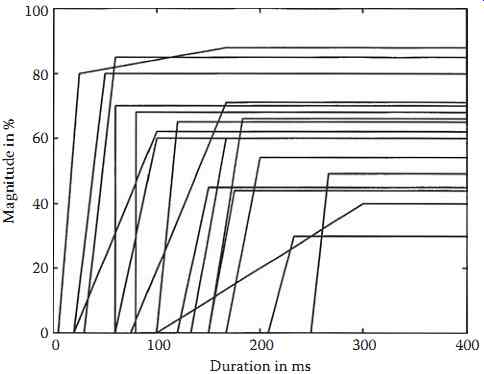
FIG. 8 Voltage-tolerance performance for personal computers.
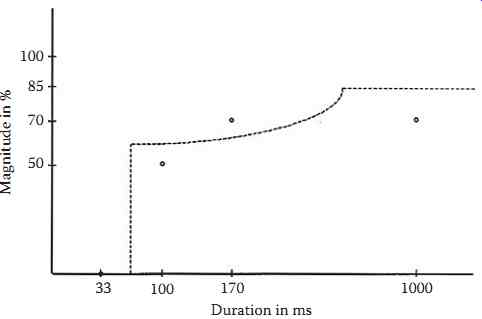
FIG. 9 Average voltage-tolerance curve for adjustable-speed drives.
From performance testing of adjustable-speed drives, an "average voltage-tolerance curve" has been obtained. This curve is shown in FIG. 9. The sags for which the drive was tested are indicated as circles. It has further been assumed that the drives can operate indefinitely on 85% voltage. Voltage tolerance is defined here as "automatic speed recovery, without reaching zero speed." For sensitive production processes, more strict requirements will hold.
2.3 Single-Phase Rectifiers
The sensitivity of most single-phase equipment can be understood from the equivalent scheme in FIG. 10. The power supply to a computer, process-control equipment, consumer electronics, etc. consists of a single-phase (four-pulse) rectifier together with a capacitor and a DC/DC converter. During nor mal operation the capacitor is charged twice a cycle through the diodes. The result is a DC voltage ripple:

(eqn 11)
... with P the DC bus active-power load, T one cycle of the power frequency, V0 the maximum DC bus volt age, and C the size of the capacitor.
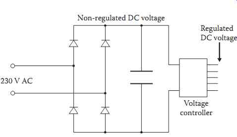
FIG. 10 Typical power supply to sensitive single-phase equipment.
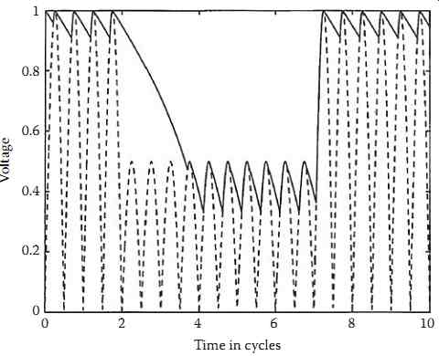
FIG. 11 Absolute value of AC voltage (dashed) and DC bus voltage (solid line)
for a sag down to 50%.
During a voltage sag or interruption, the capacitor continues to discharge until the DC bus volt age has dropped below the peak of the supply voltage. A new steady state is reached, but at a lower DC bus voltage and with a larger ripple. The resulting DC bus voltage for a sag down to 50% is shown in FIG. 11, together with the absolute value of the supply voltage. If the new steady state is below the minimum operating voltage of the DC/DC converter, or below a certain protection setting, the equipment will trip. During the decaying DC bus voltage, the capacitor voltage V(t) can be obtained from the law of conservation of energy:
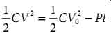
(eqn 12)
where a constant DC bus load P has been assumed. From Equation 12 the voltage as a function of time is obtained:
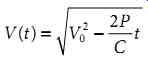
(eqn 13)
Combining this with Equation 11 gives the following expression:
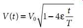
(eqn 14)
The larger the DC ripple in normal operation, the faster the drop in DC bus voltage during a sag. From Equation 14 the maximum duration of zero voltage tmax is calculated for a minimum operating volt age Vmin, resulting in
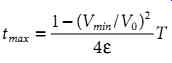
(eqn 15)
2.4 Three-Phase Rectifiers
The performance of equipment fed through three-phase rectifiers becomes somewhat more complicated. The main equipment belonging to this category is formed by AC and DC adjustable-speed drives.
One of the complications is that the operation of the equipment is affected by the three voltages, which are not necessarily the same during the voltage sag. For non-controlled (six pulse) diode rectifiers, a similar model can be used as for single-phase rectifiers. The operation of three-phase controlled rectifiers can become very complicated and application-specific. Therefore, only noncontrolled rectifiers will be discussed here. For voltage sags due to three-phase faults, the DC bus voltage behind the (three-phase) rectifier will decay until a new steady state is reached at a lower voltage level, with a larger ripple. To calculate the DC bus voltage as a function of time, and the time-to-trip, the same equation as for the single-phase rectifier can be used.
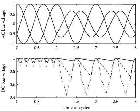
FIG. 12 AC and DC side voltages for a three-phase rectifier during a sag of
type C.
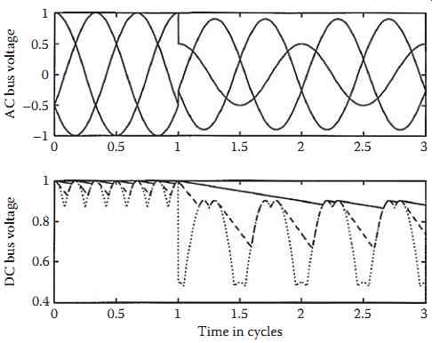
FIG. 13 AC and DC side voltages for a three-phase rectifier during a sag of
type D.
For unbalanced voltage sags, a distinction needs to be made between the two types (C and D), as introduced in Section 38.1.8. FIG. 12 shows AC and DC side voltages for a sag of type C with V = 0.5 pu and F = 1. For this sag, the voltage drops in two phases where the third phase stays at its presage value. Three capacitor sizes are used; a "large" capacitance is defined as a value that leads to an initial decay of the DC voltage equal to 10%, which is 433 F/kW for a 620 V drive. In the same way, "small" capacitance corresponds to 75% per cycle initial decay, and 57.8 F/kW for a 620 V drive. It turns out that even for the small capacitance, the DC bus voltage remains above 70%. For the large capacitance value, the DC bus voltage is hardly affected by the voltage sag. It is easy to understand that this is also the case for type C sags with an even lower characteristic magnitude V.
FIG. 13 shows the equivalent results for a sag of type D, again with V = 0.5 and F = 1. As all three AC voltages show a drop in voltage magnitude, the DC bus voltage will drop even for a large capacitor.
But the effect is still much less than for a three-phase (balanced) sag.
The effect of a lower PN factor (F < 1) is that even the highest voltage shows a drop for a type C sag, so that the DC bus voltage will always show a small drop. Also for a type D sag, a lower PN factor will lead to an additional drop in DC bus voltage.
3. Mitigation of Voltage Sags
3.1 From Fault to Trip
To understand the various ways of mitigation, the mechanism leading to an equipment trip needs to be understood. The equipment trip is what makes the event a problem; if there are no equipment trips, there is no voltage sag problem. The underlying event of the equipment trip is a short-circuit fault. At the fault position, the voltage drops to zero, or to a very low value. This zero voltage is changed into an event of a certain magnitude and duration at the interface between the equipment and the power system. The short-circuit fault will always cause a voltage sag for some customers. If the fault takes place in a radial part of the system, the protection intervention clearing the fault will also lead to an interruption. If there is sufficient redundancy present, the short circuit will only lead to a voltage sag. If the resulting event exceeds a certain severity, it will cause an equipment trip.
Based on this reasoning, it is possible to distinguish between the following mitigation methods:
• Reducing the number of short-circuit faults.
• Reducing the fault-clearing time.
• Changing the system such that short-circuit faults result in less severe events at the equipment terminals or at the customer interface.
• Connecting mitigation equipment between the sensitive equipment and the supply.
• Improving the immunity of the equipment.
3.2 Reducing the Number of Faults
Reducing the number of short-circuit faults in a system not only reduces the sag frequency, but also the frequency of long interruptions. This is thus a very effective way of improving the quality of supply and many customers suggest this as the obvious solution when a voltage sag or interruption problem occurs. Unfortunately, most of the time the solution is not that obvious. A short circuit not only leads to a voltage sag or interruption at the customer interface, but may also cause damage to utility equipment and plant. Therefore, most utilities will already have reduced the fault frequency as far as economically feasible. In individual cases, there could still be room for improvement, e.g., when the majority of trips are due to faults on one or two distribution lines. Some examples of fault mitigation are:
• Replace overhead lines by underground cables.
• Use special wires for overhead lines.
• Implement a strict policy of tree trimming.
• Install additional shielding wires.
• Increase maintenance and inspection frequencies.
One has to keep in mind, however, that these measures can be very expensive, especially for transmission systems, and that their costs have to be weighted against the consequences of the equipment trips.
3.3 Reducing the Fault-Clearing Time
Reducing the fault-clearing time does not reduce the number of events, but only their severity. It does not do anything to reduce to number of interruptions, but can significantly limit the sag duration. The ultimate reduction of fault-clearing time is achieved by using current-limiting fuses, able to clear a fault within one half-cycle. The recently introduced static circuit breaker has the same characteristics: fault-clearing time within one half-cycle. Additionally, several types of fault-current limiters have been proposed that do not actually clear the fault, but significantly reduce the fault current magnitude within one or two cycles. One important restriction of all these devices is that they can only be used for low- and medium-voltage systems. The maximum operating voltage is a few tens of kilovolts.
But the fault-clearing time is not only the time needed to open the breaker, but also the time needed for the protection to make a decision. To achieve a serious reduction in fault-clearing time, it is necessary to reduce any grading margins, thereby possibly allowing for a certain loss of selectivity.
3.4 Changing the Power System
By implementing changes in the supply system, the severity of the event can be reduced. Here again, the costs may become very high, especially for transmission and subtransmission voltage levels. In industrial systems, such improvements more often outweigh the costs, especially when already included in the design stage. Some examples of mitigation methods especially directed toward voltage sags are
• Install a generator near the sensitive load. The generators will keep up the voltage during a remote sag. The reduction in voltage drop is equal to the percentage contribution of the generator station to the fault current. In case a combined-heat-and-power station is planned, it is worth it to consider the position of its electrical connection to the supply.
• Split buses or substations in the supply path to limit the number of feeders in the exposed area.
• Install current-limiting coils at strategic places in the system to increase the "electrical distance" to the fault. The drawback of this method is that this may make the event worse for other customers.
• Feed the bus with the sensitive equipment from two or more substations. A voltage sag in one substation will be mitigated by the infeed from the other substations. The more independent the substations are, the more the mitigation effect. The best mitigation effect is by feeding from two different transmission substations. Introducing the second infeed increases the number of sags, but reduces their severity.
3.5 Installing Mitigation Equipment
The most commonly applied method of mitigation is the installation of additional equipment at the system-equipment interface. Also recent developments point toward a continued interest in this way of mitigation. The popularity of mitigation equipment is explained by it being the only place where the customer has control over the situation. Both changes in the supply as well as improvement of the equipment are often completely outside of the control of the end user. Some examples of mitigation equipment are
• Uninterruptable power supply (UPS). This is the most commonly used device to protect low-power equipment (computers, etc.) against voltage sags and interruptions. During the sag or interruption, the power supply is taken over by an internal battery. The battery can supply the load for, typically, between 15 and 30 min.
• Static transfer switch. A static transfer switch switches the load from the supply with the sag to another supply within a few milliseconds. This limits the duration of a sag to less than one half cycle, assuming that a suitable alternate supply is available.
• Dynamic voltage restorer (DVR). This device uses modern power electronic components to insert a series voltage source between the supply and the load. The voltage source compensates for the voltage drop due to the sag. Some devices use internal energy storage to make up for the drop in active power supplied by the system. They can only mitigate sags up to a maximum duration.
Other devices take the same amount of active power from the supply by increasing the current.
These can only mitigate sags down to a minimum magnitude. The same holds for devices boosting the voltage through a transformer with static tap changer.
• Motor-generator sets. Motor-generator sets are the classical solution for sag and interruption mitigation with large equipment. They are obviously not suitable for an office environment but the noise and the maintenance requirements are often no problem in an industrial environment.
Some manufacturers combine the motor-generator set with a backup generator; others combine it with power-electronic converters to obtain a longer ride-through time.
3.6 Improving Equipment Voltage Tolerance
Improvement of equipment voltage tolerance is probably the most effective solution against equipment trips due to voltage sags. But as a short-time solution, it is often not suitable. In many cases, a customer only finds out about equipment performance after it has been installed. Even most adjustable-speed drives have become off-the-shelf equipment where the customer has no influence on the specifications.
Only large industrial equipment is custom-made for a certain application, which enables the incorporation of voltage-tolerance requirements in the specification.
Apart from improving large equipment (drives, process-control computers), a thorough inspection of the immunity of all contactors, relays, sensors, etc. can significantly improve the voltage tolerance of the process.
3.7 Different Events and Mitigation Methods
FIG. 6 showed the magnitude and duration of voltage sags and interruptions resulting from various system events. For different events, different mitigation strategies apply.
Sags due to short-circuit faults in the transmission and subtransmission system are characterized by a short duration, typically up to 100 ms. These sags are very hard to mitigate at the source and improvements in the system are seldom feasible. The only way of mitigating these events is by improvement of the equipment or, where this turns out to be unfeasible, installing mitigation equipment. For low-power equipment, a UPS is a straightforward solution; for high-power equipment and for complete installations, several competing tools are emerging.
The duration of sags due to distribution system faults depends on the type of protection used-ranging from less than a cycle for current-limiting fuses up to several seconds for overcurrent relays in underground or industrial distribution systems. The long sag duration also enables equipment to trip due to faults on distribution feeders fed from other HV/MV substations. For deep long-duration sags, equipment improvement becomes more difficult and system improvement easier. The latter could well become the preferred solution, although a critical assessment of the various options is certainly needed.
Sags due to faults in remote distribution systems and sags due to motor starting should not lead to equipment tripping for sags down to 85%. If there are problems, the equipment needs to be improved. If equipment trips occur for long-duration sags in the 70%-80% magnitude range, changes in the system have to be considered as an option.
For interruptions, especially the longer ones, equipment improvement is no longer feasible. System improvements or a UPS in combination with an emergency generator are possible solutions here.