AMAZON multi-meters discounts AMAZON oscilloscope discounts
Power system harmonics are not a new topic, but the proliferation of high-power electronics used in motor drives and power controllers has necessitated increased research and development in many areas relating to harmonics. For many years, high-voltage direct current (HVDC) stations have been a major focus area for the study of power system harmonics due to their rectifier and inverter stations. Roughly two decades ago, electronic devices that could handle several kW up to several MW became commercially viable and reliable products. This technological advance in electronics led to the widespread use of numerous converter topologies, all of which represent nonlinear elements in the power system.
Even though the power semiconductor converter is largely responsible for the large-scale interest in power system harmonics, other types of equipment also present a nonlinear characteristic to the power system. In broad terms, loads that produce harmonics can be grouped into three main categories covering (1) arcing loads, (2) semiconductor converter loads, and (3) loads with magnetic saturation of iron cores. Arcing loads, like electric arc furnaces and florescent lamps, tend to produce harmonics across a wide range of frequencies with a generally decreasing relationship with frequency. Semiconductor loads, such as adjustable-speed motor drives, tend to produce certain harmonic patterns with relatively predictable amplitudes at known harmonics. Saturated magnetic elements, like overexcited transformers, also tend to produce certain "characteristic" harmonics. Like arcing loads, both semiconductor converters and saturated magnetics produce harmonics that generally decrease with frequency.
Regardless of the load category, the same fundamental theory can be used to study power quality problems associated with harmonics. In most cases, any periodic distorted power system waveform (voltage, current, flux, etc.) can be represented as a series consisting of a DC term and an infinite sum of sinusoidal terms as shown in Equation 1 where ω0 is the fundamental power frequency.
(eqn 1)
A vast amount of theoretical mathematics has been devoted to the evaluation of the terms in the infinite sum in Equation 1, but such rigor is beyond the scope of this chapter. For the purposes here, it is reasonable to presume that instrumentation is available that will provide both the magnitude Fi and the phase angle [theta]i for each term in the series. Taken together, the magnitude and phase of the ith term completely describe the ith harmonic.
It should be noted that not all loads produce harmonics that are integer multiples of the power frequency. These non-integer multiple harmonics are generally referred to as interharmonics and are commonly produced by arcing loads and cycloconverters. All harmonic terms, both integer and non integer multiples of the power frequency, are analytically treated in the same manner, usually based on the principle of superposition.
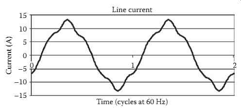
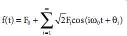
FIG. 1 Current waveform.
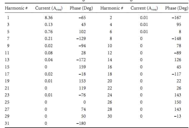
TABLE 1 Current Harmonic Magnitudes and Phase Angles
FIG. 2 Harmonic magnitude spectrum.
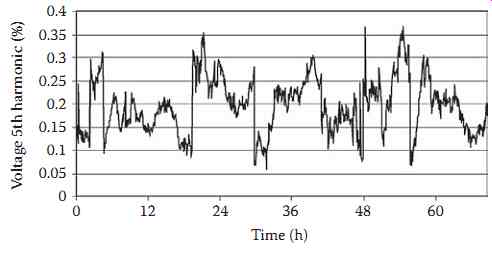
FIG. 3 Example of time-varying nature of harmonics.
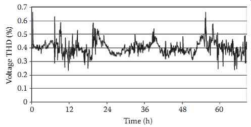
FIG. 4 Example of time-varying nature of voltage THD.
In practice, the infinite sum in Equation 1 is reduced to about 50 terms; most measuring instruments do not report harmonics higher than the 50th multiple (2500-3000 Hz for 50-60 Hz systems). The reporting can be in the form of a tabular listing of harmonic magnitudes and angles or in the form of a magnitude and phase spectrum. In each case, the information provided is the same and can be used to reproduce the original waveform by direct substitution into Equation 1 with satisfactory accuracy.
As an example, FIG. 1 shows the (primary) current waveform drawn by a small industrial plant.
Table 1 shows a table of the first 31 harmonic magnitudes and angles. FIG. 2 shows a bar graph magnitude spectrum for this same waveform. These data are widely available from many commercial instruments; the choice of instrument makes little difference in most cases.
A fundamental presumption when analyzing distorted waveforms using Fourier methods is that the waveform is in steady state. In practice, waveform distortion varies widely and is dependent on both load levels and system conditions. It is typical to assume that a steady-state condition exists at the instant at which the measurement is taken, but the next measurement at the next time could be markedly different. As examples, Figures 3 and 4 show time plots of fifth harmonic voltage and the total harmonic distortion, respectively, of the same waveform measured on a 115 kV transmission system near a 5 MW customer. Note that the THD is fundamentally defined in Equation 2, with 50 often used in practice as the upper limit on the infinite summation.
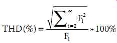
(eqn 2)
Because harmonic levels are never constant, it is difficult to establish utility-side or manufacturing side limits for these quantities. In general, a probabilistic representation is used to describe harmonic quantities in terms of percentiles. Often, the 95th and 99th percentiles are used for design or operating limits. FIG. 5 shows a histogram of the voltage THD in FIG. 4, and also includes a cumulative probability curve derived from the frequency distribution. Any percentile of interest can be readily calculated from the cumulative probability curve.
Both the Institute of Electrical and Electronics Engineers (IEEE) and the International Electrotechnical Commission (IEC) recognize the need to consider the time-varying nature of harmonics when deter mining harmonic levels that are permissible. Both organizations publish harmonic limits, but the degree to which the various limits can be applied varies widely. Both IEEE and IEC publish "system-level" harmonic limits that are intended to be applied from the utility point-of-view in order to limit power system harmonics to acceptable levels. The IEC, however, goes further and also publishes harmonic limits for individual pieces of equipment.
The IEEE limits are covered in two documents, IEEE 519-1992 and IEEE 519A (draft). These documents suggest that harmonics in the power system be limited by two different methods. One set of harmonic limits is for the harmonic current that a user can inject into the utility system at the point where other customers are or could be (in the future) served. (Note that this point in the system is often called the point of common coupling, or PCC.) The other set of harmonic limits is for the harmonic voltage that the utility can supply to any customer at the PCC. With this two-part approach, customers insure that they do not inject an "unreasonable" amount of harmonic current into the system, and the utility insures that any "reasonable" amount of harmonic current injected by any and all customers does not lead to excessive voltage distortion.
Table 2 shows the harmonic current limits that are suggested for utility customers. The table is broken into various rows and columns depending on harmonic number, short circuit to load ratio, and voltage level. Note that all quantities are expressed in terms of a percentage of the maximum demand current (IL in the table). Total demand distortion (TDD) is defined to be the rms value of all harmonics, in amperes, divided by the maximum (12 month) fundamental frequency load current, IL, with this ratio then multiplied by 100%.
The intent of the harmonic current limits is to permit larger customers, who in concept pay a greater share of the cost of power delivery equipment, to inject a greater portion of the harmonic current (in amperes) that the utility can absorb without producing excessive voltage distortion. Furthermore, customers served at transmission level voltage have more restricted injection limits than do customers served at lower voltage because harmonics in the high voltage network have the potential to adversely impact a greater number of other users through voltage distortion.
Table 3 gives the IEEE 519-1992 voltage distortion limits. Similar to the current limits, the permissible distortion is decreased at higher voltage levels in an effort to minimize potential problems for the majority of system users. Note that Tables 2 and 3 are given here for illustrative purposes only; the reader is strongly advised to consider additional material listed at the end of this chapter prior to trying to apply the limits.
The IEC formulates similar limit tables with the same intent: limit harmonic current injections so that voltage distortion problems are not created; the utility will correct voltage distortion problems if they exist and if all customers are within the specified harmonic current limits. Because the numbers suggested by the IEC are similar (but not identical) to those given in Tables 2 and 3, the IEC tables for system-level harmonic limits given in IEC 1000-3-6 are not repeated here.
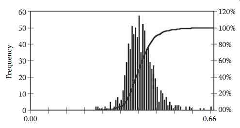
FIG. 5 Probabilistic representation of voltage THD.
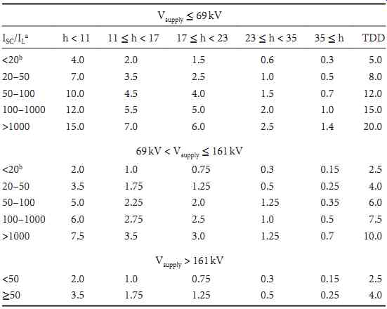
TABLE 2 IEEE-519 Harmonic Current Limits
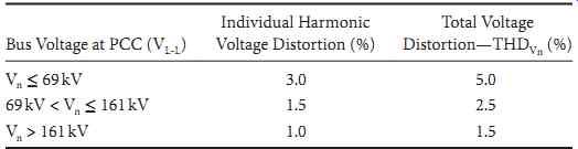
TABLE 3 IEEE 519-1992 Voltage Harmonic Limits
While the IEEE harmonic limits are designed for application at the three-phase PCC, the IEC goes further and provides limits appropriate for single-phase and three-phase individual equipment types.
The most notable feature of these equipment limits is the "mA per W" manner in which they are pro posed. For a wide variety of harmonic-producing loads, the steady-state (normal operation) harmonic currents are limited by prescribing a certain harmonic current, in mA, for each watt of power rating.
The IEC also provides a specific waveshape for some load types that represents the most distorted cur rent waveform allowed. Equipment covered by such limits include personal computers (power supplies) and single-phase battery charging equipment.
Even though limits exist, problems related to harmonics often arise from single, large "point source" harmonic loads as well as from numerous distributed smaller loads. In these situations, it is necessary to conduct a measurement, modeling, and analysis campaign that is designed to gather data and develop a solution. As previously mentioned, there are many commercially available instruments that can provide harmonic measurement information both at a single "snapshot" in time as well as continuous monitoring over time. How this information is used to develop problem solutions, however, can be a very complex issue.
Computer-assisted harmonic studies generally require significantly more input data than load flow or short circuit studies. Because high frequencies (up to 2-3 kHz) are under consideration, it is important to have mathematically correct equipment models and the data to use in them. Assuming that this data is available, there are a variety of commercially available software tools for actually performing the studies.
Most harmonic studies are performed in the frequency domain using sinusoidal steady-state techniques. (Note that other techniques, including full time-domain simulation, are sometimes used for specific problems.) A power system equivalent circuit is prepared for each frequency to be analyzed (recall that the Fourier series representation of a waveform is based on harmonic terms of known frequencies), and then basic circuit analysis techniques are used to determine voltages and currents of interest at that frequency. Most harmonic producing loads are modeled using a current source at each frequency that the load produces (arc furnaces are sometimes modeled using voltage sources), and network currents and voltages are determined based on these load currents. Recognize that at each frequency, voltage and current solutions are obtained from an equivalent circuit that is valid at that frequency only; the principle of superposition is used to "reconstruct" the Fourier series for any desired quantity in the network from the solutions of multiple equivalent circuits. Depending on the software tool used, the results can be presented in tabular form, spectral form, or as a waveform as shown in Table 1 and Figures 1 and 2, respectively. An example voltage magnitude spectrum obtained from a harmonic study of a distribution primary circuit is shown in FIG. 6.
Regardless of the presentation format of the results, it is possible to use this type of frequency-domain harmonic analysis procedure to predict the impact of harmonic producing loads at any location in any power system. However, it is often impractical to consider a complete model of a large system, especially when unbalanced conditions must be considered. Of particular importance, however, are the locations of capacitor banks.
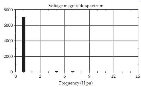
FIG. 6 Sample magnitude spectrum results from a harmonic study.
When electrically in parallel with network inductive reactance, capacitor banks produce a parallel resonance condition that tends to amplify voltage harmonics for a given current harmonic injection.
When electrically in series with network inductive reactance, capacitor banks produce a series resonance condition that tends to amplify current harmonics for a given voltage distortion. In either case, harmonic levels far in excess of what are expected can be produced. Fortunately, a relatively simple calculation procedure called a frequency scan, can be used to indicate potential resonance problems. FIG. 7 shows an example of a frequency scan conducted on the positive sequence network model of a distribution circuit. Note that the distribution primary included the standard feeder optimization capacitors.
A frequency scan result is actually a plot of impedance vs. frequency. Two types of results are avail able: driving point and transfer impedance scans. The driving point frequency scan shown in FIG. 7 indicates how much voltage would be produced at a given bus and frequency for a 1 A current injection at that same location and frequency. Where necessary, the principle of linearity can be used to scale the 1 A injection to the level actually injected by specific equipment. In other words, the driving point impedance predicts how a customer's harmonic producing load could impact the voltage at that load's terminals. Local maximums, or peaks, in the scan plot indicate parallel resonance conditions. Local minimums, or valleys, in the scan plot indicate series resonance.
A transfer impedance scan predicts how a customer's harmonic producing load at one location can impact voltage distortions at other (possibly very remote) locations. In general, to assess the ability of a relatively small current injection to produce a significant voltage distortion (due to resonance) at remote locations (due to transfer impedance) is the primary goal of every harmonic study.
Should a harmonic study indicate a potential problem (violation of limits, for example), two categories of solutions are available: (1) reduce the harmonics at their point of origin (before they enter the system), or (2) apply filtering to reduce undesirable harmonics. Many methods for reducing harmonics at their origin are available; for example, using various transformer connections to cancel certain harmonics has been extremely effective in practice. In most cases, however, reducing or eliminating harmonics at their origin is effective only in the design or expansion stage of a new facility. For existing facilities, harmonic filters often provide the least-cost solution.
Harmonic filters can be subdivided into two types: active and passive. Active filters are only now becoming commercially viable products for high-power applications and operate as follows. For a load that injects certain harmonic currents into the supply system, a DC to AC inverter can be controlled such that the inverter supplies the harmonic current for the load, while allowing the power system to supply the power frequency current for the load. FIG. 8 shows a diagram of such an active filter application.
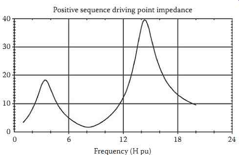
FIG. 7 Sample frequency scan results.
===
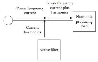
FIG. 8 Active filter concept diagram.
- Power frequency current
- Current harmonics
- Power frequency current plus harmonics
- Harmonic producing load
- Active filter
===
For high power applications or for applications where power factor correction capacitors already exist, it is typically more cost effective to use passive filtering. Passive filtering is based on the series resonance principle (recall that a low impedance at a specific frequency is a series-resonant characteristic) and can be easily implemented. FIG. 9 shows a typical three-phase harmonic filter (many other designs are also used) that is commonly used to filter fifth or seventh harmonics.
It should be noted that passive filtering cannot always make use of existing capacitor banks. In filter applications, the capacitors will typically be exposed continuously to voltages greater than their ratings (which were determined based on their original application). 600V capacitors, for example, may be required for 480V filter applications. Even with the potential cost of new capacitors, passive filtering still appears to offer the most cost effective solution to the harmonic problem at this time.
In conclusion, power system harmonics have been carefully considered for many years and have received a significant increase in research and development activity as a direct result of the proliferation of high-power semiconductors. Fortunately, harmonic measurement equipment is readily available, and the underlying theory used to evaluate harmonics analytically (with computer assistance) is well understood. Limits for harmonic voltages and currents have been suggested by multiple standards-making bodies, but care must be used because the suggested limits are not necessarily equivalent.
Regardless of which limit numbers are appropriate for a given application, multiple options are avail able to help meet the levels required. As with all power quality problems, however, accurate study on the "front end" usually will reveal possible problems in the design stage, and a lower-cost solution can be implemented before problems arise.
The material presented here is not intended to be all-inclusive. The suggested reading provides further documents, including both IEEE and IEC standards, recommended practices, and technical papers and reports that provide the knowledge base required to apply the standards properly.
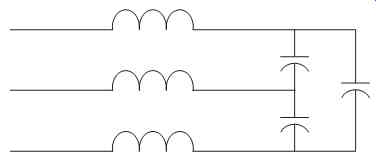
FIG. 9 Typical passive filter design.