AMAZON multi-meters discounts AMAZON oscilloscope discounts
1. Introduction
The appearance of the first transmission lines more than 100 years ago immediately started discussion and public concerns. When the first transmission line was built, more electrocutions occurred because of people climbing up the towers, flying kites, and touching wet conducting ropes. As the public became aware of the danger of electrocution, the aesthetic effect of the transmission lines generated public discussion. In fact, there is a story of Frank Lloyd Wright, the famous architect, calling President Roosevelt and demanding the removal of high-voltage lines obstructing his view in Scottsdale, Arizona.
Undoubtedly, a transmission line corridor with several lines would disturb the appearance of a quite green valley.
The rapid increase in radio and television transmission has produced the occurrence of electromagnetic interference (EMI) problems. The high voltage on the transmission line produces corona discharge that generates electromagnetic waves. These waves disturb the radio and television reception, which resulted in public protests and opposition to build lines too near towns.
In the 1960s, the electrical field surrounding the high-voltage lines became subject to public concerns.
The electrical field can produce minor sparks and small electric shocks under a high-voltage line. An example of this would be if a woman were to walk under a line holding an umbrella, the woman would feel the electric shocks produced by these small discharges.
In the 1970s, the transmission line current produced magnetic fields and became a public issue.
Several newspaper articles discussed the adverse health effects of magnetic fields. This generated intensive research all over the world. The major concern is that exposure to magnetic fields caused cancer, mostly leukemia. The U.S. government report concluded that there was no evidence that moderate 60 Hz magnetic field caused cancer. However, this opinion is not shared by all.
This section will discuss the listed environmental effects of transmission lines.
2. Aesthetic Effects of Lines
The first transmission towers were small wooden poles that were tempting for children to climb but had no environmental impact. However, the increase of voltage resulted in large steel structures over 100 ft high and 50 ft wide.
In North America, the large wooden structures were common until the Second World War. The typical voltage of transmission lines with wooden poles is less than 132 kV, although 220 kV lines with H-frame wooden towers are also built in the Midwest.
FIG. 1 shows a transmission line with H-frame wooden towers. This construction fits well in the rural environment and does not produce environmental concerns.
The increasing voltage and need for crossing large valleys and rivers resulted in the appearance of steel towers. These towers are welded or riveted lattice structures. Several different conductor arrangements are used. FIG. 2a shows a lattice tower with conductors arranged horizontally. The horizontal arrangement increases the widths of the tower, which produces a more visible effect. FIG. 2b shows a double circuit line with vertically arranged conductors. This results in a taller and more compact appearance.
The presented pictures demonstrate that the transmission lines with large steel towers are not very aesthetically pleasing. They do not blend in with the environment and can interrupt a beautiful landscape.
The increasing demand of electricity and the public objection to build new transmission lines resulted in the development of transmission line corridors. The utilities started to build lines in parallel on right-of-ways land that they already owned. FIG. 3 shows a typical transmission line corridor. The appearance of the maze of conductors and large steel structures are not an aesthetically pleasing sight.
The public displeasure with the lattice tower triggered research work on the development of aesthetically more pleasing structures. Several attempts were made to develop nonmetallic transmission line structure using fiberglass rods, where the insulators are replaced by the tower itself. Although the development of nonmetallic structures was unsuccessful, the development of tubular steel towers led to a more pleasing appearance. FIG. 4 shows tubular steel tower used in Arizona at the 220 kV high voltage lines.
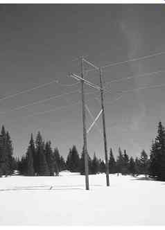
FIG. 1 220 kV line with H-frame wooden towers.
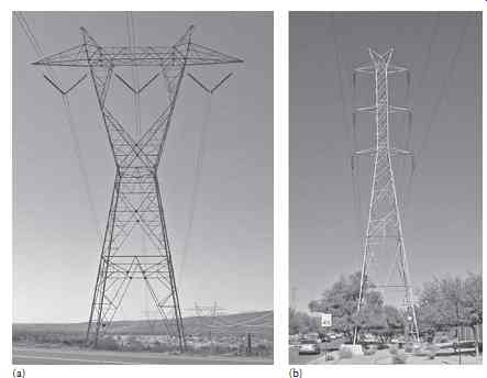
FIG. 2 High-voltage transmission lines. (a) Single circuit line with
horizontally arranged conductors. (b) Double circuit line with
vertically arranged conductors.
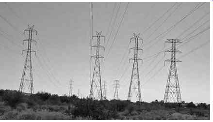
FIG. 3 Transmission line corridor.
FIG. 4 demonstrates that the slender tubular structure is less disturbing and aesthetically more pleasing. These towers blend in better with the desert environment and cause less visual interruptions.
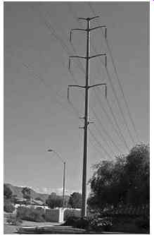
FIG. 4 A 220 kV suspension tower.
The presented examples prove that the aesthetic appearance of the transmission lines is improving although even the best tower structures disturb the environment. The ultimate solution is the replacement of the lines by an underground cable system. Unfortunately, both technical and economic problems are preventing the use of underground energy transmission systems.
3. Magnetic Field Generated by HV Lines
Several newspaper articles presented survey results showing that the exposure to magnetic fields increases the cancer occurrence. Studies linked the childhood leukemia to transmission line-generated magnetic field exposure. This triggered research in both biological and electrical engineering fields.
The biological research studied the magnetic field effect on cells and performed statistical studies to determine the correlation between field exposure and cancer occurrence. The electrical engineering research aimed at the determination of magnetic field strength near transmission lines, electric equipment, motors, and appliances. A related engineering problem is the reduction of magnetic field generated by lines and other devices.
In this section we will present a calculation method to determine a transmission line-generated magnetic field and summarize the major results of biological research.
3.1 Magnetic Field Calculation
The electric current in a cylindrical transmission line conductor generates magnetic field surrounding the conductor. The magnetic field lines are concentric circles. At each point around the conductor, the magnetic field strength or intensity is described by a field vector that is perpendicular to the radius drawn from the center of the conductor.
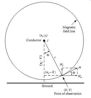
FIG. 5 Magnetic field generation.
FIG. 5 shows the current-carrying conductor, a circular magnetic field line, and the magnetic field vector H in a selected observation point. The magnetic field vector is perpendicular to the radius of the circular magnetic field line. The H field vector is divided into horizontal and vertical components.
The location of both the observation point and the conductor is described by the x, y coordinates.
The magnetic field intensity is calculated by using the ampere law. The field intensity is:
...where...
H is the field intensity in A/m
I is the current in the conductor
r is the distance from the conductor
(X, Y) are the coordinates of the observation point
(xi , yi ) are the coordinates of the conductor
The horizontal and vertical components of the field are calculated from the triangle formed by the field vectors. The angle is calculated from the triangle formed with the coordinate's differences as shown in FIG. 5:
In a three-phase system, each of the three-phase currents generates magnetic fields. The phase currents and corresponding field vectors are shifted by 120°. The three-phase currents are:
The three-phase-line-generated field intensity is calculated by substituting the conductor currents and coordinates in the equations describing the horizontal and vertical field components. This produces three horizontal and three vertical field vectors. The horizontal and vertical components of the three phase-line-generated magnetic field are the sum of the three-phase components:
[...]
...where ...
Hx is the horizontal component of three-phase-generated magnetic field
Hy is the vertical component of three-phase-generated magnetic field
Hx_1, Hx_2, Hx_3 are the horizontal components of phases 1, 2, and 3 generated magnetic field
Hy_1, Hy_2, Hy_3 are the vertical components of phases 1, 2, and 3 generated magnetic field
The vector sum of the horizontal and vertical components gives the three-phase-line-generated total magnetic field intensity:
The magnetic field flux density is calculated by multiplying the field intensity by the free space permeability:
For the demonstration of the expected results, we calculated a 500 kV transmission line-generated magnetic flux density under the line in 1 m distance from the ground. The conductors are arranged horizontally. The average conductor height is 24.38 m (80 ft); the distance between the conductors is 10.66 m (35 ft). The line current is 2000 A. FIG. 6 shows the magnetic flux density distribution under the line in 1 m from the ground. The locations of the line conductors are marked on the figure. It can be seen that the maximum flux density is under the middle conductor and it decreases rapidly with distance.
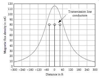 FIG. 6 Magnetic field density under a 500 kV line when the load current
is 2000 A.
FIG. 6 Magnetic field density under a 500 kV line when the load current
is 2000 A.
The right-of-way is around 200 ft in this transmission line. The maximum flux density is around 116 mG (milligauss) or 11.6 µT and around 18 mG (1.8 µT) at the edge of the right-of-way.
Although the acceptable level of magnetic flux density is not specified by national or international standards, the utilities maintain less than 100 mG (10 µT) at the edge of the right-of-way and less than 10 mG (1 µT) at the neighboring residential area.
3.2 Health Effect of Magnetic Field
The health effects of magnetic fields are a controversial subject, which generated an emotional discussion. The first study that linked the occurrence of childhood leukemia to electrical current-generated magnetic fields was published in 1979 by Wertheimer and Leeper. This was a statistical study where the electric wiring configuration near the house of the victim was related to the occurrence of child hood cancer. The researchers compared the wiring of the configuration including transmission lines close to the childhood leukemia victim's house and close to the house of a controlled population group.
The study found a correlation between the occurrence of cancer and the power lines carrying high cur rent. The study was dismissed because of inconsistencies and repeated in 1988 by Savitz et al.. They measured the magnetic field in the victim's house and used the electric wiring configuration. The study found a modest statistical correlation between the cancer and wiring code but not between the cancer and the measured magnetic field. These findings initiated worldwide research on magnetic field health effects. The studies can be divided into three major categories:
• Epidemiological studies
• Laboratory studies
• Exposure assessment studies
3.2.1 Epidemiological Studies
These statistical studies connect the exposure to magnetic and electric fields to health effects, particularly to occurrence of cancer. The early studies investigated the childhood cancer occurrence and residential wiring. This was followed by studies relating the occupation (electrical worker) to cancer occurrence. In this category, the most famous one is a Swedish study, which found elevated risk for lymphoma among electric workers. However, other studies found no elevated cancer risk. The uncertainty in all of these studies is the assessment of actual exposure to electromagnetic fields. As an example, some of the studies estimated the exposure to magnetic field using the job title of the worker or the postal code where the worker lived. The results of these studies are inconclusive, some of the studies showed elevated risk to cancer, most of them not.
3.2.2 Laboratory Studies
These studies are divided into two categories-tissue studies and live animal studies. The tissue studies investigated the effect of electric and magnetic field on animal tissues. The studies showed that the electromagnetic field could cause chromosomal changes, single strand breaks, or alteration of ornithine decarboxylase, etc.. Some of the studies speculate that the electromagnetic exposure can be a promoter of cancer together with other carcinogen material. The general conclusion is that the listed effects do not prove that the EMF can be linked to cancer or other health effects.
The study on live animals showed behavioral changes in rats and mice. Human studies observed changes of heart rates and melatonin production as a result of EMF exposure. The problem with the laboratory studies are that they use a much higher field than what occurs in residential areas. None of these studies showed that the EMF produces toxicity that is typical for carcinogens. An overall conclusion is that laboratory studies cannot prove that magnetic fields are related to cancer in humans.
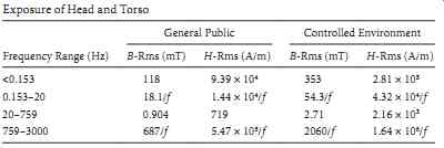
TABLE 1 Magnetic Maximum Permissible Exposure (MPE) Levels: Exposure
of Head and Torso
3.2.3 Exposure Assessment Studies
In the United States, the Electrical Power Research Institute led the research effort to assess the exposure to magnetic fields. One of the interesting conclusions is the effect of ground current flowing through main water pipes. This current can generate a significant portion of magnetic fields in a residential area.
Typically in 1 m distance from a TV, the magnetic field can be 0.01-0.2 µT; an electric razor and a fluorescent table lamp can produce a maximum of 0.3 µT. The worst is the microwave oven that can produce magnetic field around 0.3-0.8 µT in 1 m distance. The electric field produced by appliances varies between 30 and 130 V/m in a distance of 30 cm. The worst is the electric blanket that may generate 250 V/m.
The measurement of magnetic fields also created problems. EPRI developed a movable magnetic field measuring instrument. IEEE developed a standard ANSI/IEEE Std. 644 that presents a procedure to measure electric and magnetic field emitted by power lines. The conclusion is that both measuring techniques and instruments provide accurate exposure measurement.
The permitted maximum exposure to magnetic fields depends on the flux density and frequency.
International Commission on Non-Ionizing Radiation Protection (ICNIRP) guidelines of the reference levels for exposure to time varying 60 Hz magnetic fields are
• 833 mG for the general public
• 4167 G for the work environment
Institute of Electrical and Electronics Engineers (IEEE) Standard C95.6 provides the maximum EMF permissible exposure levels for the human body in the general public and in controlled environments.
The permissible magnetic flux density and magnetic field values are listed in TABLE 1.
The IEEE standards are approximately an order of magnitude higher than the ICNIRP reference levels. A consensus has not been reached about health risks, and some individual scientists have proposed more restrictive exposure guidelines.
3.2.4 Summary
The health effect of magnetic field remains a controversial topic in spite of the U.S. Environmental Protection Agency report that concluded that the low frequency, low level electric, and magnetic fields are not producing any health risks.
Many people believe that the prudent approach is the "prudent avoidance" to long-term exposure.
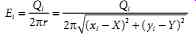
4. Electrical Field Generated by HV Lines
The energized transmission line produces electric field around the line. The high voltage on a transmission line drives capacitive current through the line. Typically, the capacitive current is maximum at the supply and linearly reduced to zero at the end of a no-loaded line, because of the evenly distributed line capacitance. The capacitive current generates sinusoidal variable charges on the conductors. The rms value of the sinusoidal charge is calculated and expressed as coulomb per meter. The equations describing the relation between the voltage and charge were derived in section 21. For a better understanding, we summarize the derivation of equations for field calculation.
FIG. 7 shows a long energized cylindrical conductor. This conductor generates an electrical field.
The emitted electrical field lines are radial and the field inside the conductor is zero. The electric field intensity is:
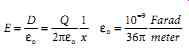
...where D is the electric field flux density
eo is the free place permeability
Q is the charge on the conductor
x is the radial distance
E is the electric field intensity
The integral of the electric field between two points gives the voltage differences:
Typically, the three-phase transmission line is built with three conductors placed above the ground.
The voltage between the conductors is the line-to-line voltage and between the conductor and ground is the line-to-ground voltage. As we described before, the line energization generates charges on the conductors. The conductor charges produce an electric field around the conductors. The electric field lines are radial close to the conductors. In addition to the electrical field, the conductor is surrounded by equipotential lines. The equipotential lines are circles in case of one conductor above the ground. The voltage difference between the conductor and the equipotential line is constant.
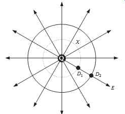
FIG. 7 A charge-generated electric field.
From a practical point of view, the voltage difference between a point in the space and the ground is important. This voltage difference is called space potential. FIG. 8 shows the electric field lines and equipotential lines for a charged conductor aboveground.
4.1 Electric Charge Calculation
FIG. 9 shows a three-phase, horizontally arranged transmission line. The ground in this figure is represented by the negatively charged image conductors. This means that each conductor of the line is represented by a positively charged line and a negatively charged image conductor. The voltage difference between the phase conductor and the corresponding image conductor is 2Vln. The electric charge on an energized conductor is calculated by repetitive use of the voltage difference equation presented before.
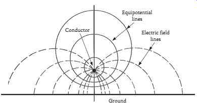
FIG. 8 Electric field around an energized conductor above the ground.
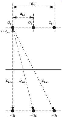
FIG. 9 Representation of three-phase-line-generated electric field by
image conductors.
The voltage difference between phase conductor "A" and its image conductor is generated by all charges (Qa, Qb, Qc, and -Qa, -Qb, -Qc) in the system. Using the voltage difference equations, we obtained the voltage difference between conductor A and its image:
Further simplification is the division of both sides of the equation by two, which results in an equation for the line to neutral voltage. Similar equations can be derived for phases B and C. The results are ...
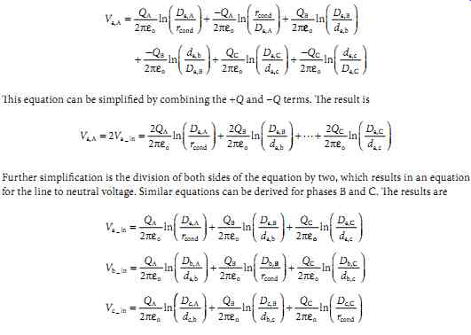
In these equations, the line to neutral voltages and dimensions are given. The equations can be solved for the charges (Qa, Qb, Qc).
4.2 Electric Field Calculation
The horizontal and vertical components of the electric field generated by the six charges (Qa, Qb, Qc, and -Qa, -Qb, -Qc) are calculated. The sum of the horizontal components and vertical components gives the X and Y components of the total electric field. The vector sum of the X and Y components gives the magnitude of the total field.
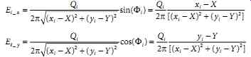
FIG. 10 shows a Q charge-generated electric field. The field lines are radial to the charge.
The absolute value of electric field generated by a charge Q is described by the Gauss equation. The observation point coordinates are X and Y. The conductor coordinates are xi and yi.
The electric field magnitude is:
The F angle between the E vector and its vertical components is:

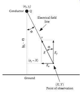
FIG. 10 Electric field generated by a charge in an observation point
(X, Y).
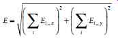
The horizontal and vertical components of the electric field are
The x and y components generated by all six charges are calculated using the previous equations.
The magnitude of the total electric field is calculated by the summation of the components. The magnitude of the total field is:
For the demonstration of the expected results, we calculated a 500 kV transmission line-generated electric field magnitude under the line in 1 m distance from the ground. The conductors are arranged horizontally. The average conductor height is 24.38 m (80 ft); the distance between the conductors is 10.66 m (35 ft). The line-to-ground voltage is
FIG. 11 shows the electric field distribution under the line in 1 m from the ground. The locations of the line conductors are marked on the figure. It can be seen that the maximum electric field is nearly under the side conductors. The electric field under the middle conductor is less than the side conductors because of the field cancellation caused by the 120° phase shift of the line voltages. The electric field decreases rapidly with the distance.
Typically, the electric field under high-voltage transmission lines varies between 2 and 10 kV/m.
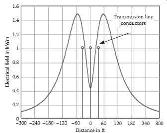
FIG. 11 Electric field under a 500 kV line.
4.3 Environmental Effect of Electric Field
In general, the electric field generated by a transmission line has no harmful health effects. Large number of studies investigated the biological effect of small 1-20 kV/m, 60 Hz electrical fields. None of the studies has shown any harmful effects. However, the electrical field can produce annoying disturbances.
The electrical field surrounding a transmission line can charge ungrounded objects close to the space potential. If the object is large, like a truck, parking under the line affects the field distribution and space potential.
The simplest visualization of the problem is a truck parking under a transmission line; the rubber tires insulate the truck from the ground. The voltage difference between the truck and the ground is determined by the capacitance between the truck and the line, and the capacitance between the truck and ground. The two capacitances form a capacitive voltage divider. The truck potential to ground can be few kilovolts. A person standing on the ground and touching the truck will discharge the capacitor between the truck and ground. This produces a small spark discharge. The person touching the truck suffers minor electric shock, which is not dangerous but uncomfortable.
After the discharge the person touching the truck grounds it, which results in a constant current through the person. This current is determined by the capacitance between the object, in this case the truck and the line. EPRI-published Redbook (Transmission Line Reference Book-345 kV and Above) gives an approximate formula for the expected current:
Icap o surface = 2pf Ey e
where
Ey is the vertical component of the electric field
f is the frequency (60 Hz)
"surface" is the equivalent charge collecting area of the object
Icap is the capacitive current flowing through the person grounding the object
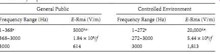
TABLE 2 Environmental Electric Field Maximum Permissible Exposure (MPE),
Whole Body Exposure
Another potentially dangerous accident scenario is when a worker climbs on a wooden ladder to repair something close to a transmission line. A grounded coworker hands him a tool. This produces a discharge and a minor spark, which is harmless. However, the shock may cause dropping the tool or falling off the ladder.
People walking under the line may experience a tingling sensation on their skin and hair stimulation if the electrical field is larger than 6-7 kV/m. This is an annoying but harmless effect.
IEEE Std C95.6 -2002 gives the maximum permissible exposure (MPE) levels for electric field. TABLE 2 shows the permissible whole body exposure levels to electric field.
The final conclusion is that the electric field should be less than 10 kV/m for the general public within the transmission line right-of-way.
5. Audible Noise
The corona discharge on the high-voltage transmission line generates audible noise. The corona discharge produced by a well-designed transmission line is very low in fair weather. Consequently, the transmission line produced audible noise in fair weather conditions is negligible.
Fog and light rain produce droplets on the surface of line conductors. The droplets increase the local electric field and generate corona discharge. The corona discharge produced air movement or pressure wave generates the audible noise. The light-rain- and fog-generated noise intensity varies, fluctuating depending on the level of wetting.
Heavy rain produces more or less constant noise. The corona discharge bursts the water droplets and disperses the water. However, the heavy rain replacing the dispersed water drops immediately.
Snowflakes also can increase corona level and audible noise. The dry, low temperature snow generally does not produce audible noise. The audible noise generated by wet melting snow can be significant and the noise level will be similar to the heavy rain-generated noise.
Typically the line-generated noise has two components:
• Broadband noise, which is mainly generated by the discharge on water droplets. This is a hissing, crackling noise with significant high-frequency components.
• Low-frequency humming noise with 120, 240 Hz, etc., components. This noise is generated by the oscillatory movement of the corona-generated ions around the conductors. The humming noise occurs mostly in good weather condition, if the line corona level is low.
From a practical point of view, the broadband noise is the most important. The utilities accept a noise level of 50-52 dB at the edge of right-of-way. The noise level is measured in dB. The base is 20 µPa.
The noise attenuates with the distance due to the divergence of the sound and the absorption of trees and other objects. Practical value is around 3 dB, when the distance is doubled.
A numerical example is presented to estimate the approximate sound level in a residential area if the sound level is 52 dB at the edge of the right-of-way. The distance between the line and the edge of right of-way is 100 ft. The sound level in a distance of 200 ft is 52 - 3 dB = 49 dB and in a distance of 400 ft is 49 - 3 dB = 46 dB.
The transmission line-generated noise level can be reduced by reduction of corona discharge level.
The most effective method is the use of bundle conductors. The rearrangement of the line conductors also can reduce corona discharge and audible noise.
The EPRI-published Transmission Line Reference Book-345 kV and Above gives curves to estimate the expected audible noise level produced by a transmission line.
6. Electromagnetic Interference
The corona discharge produces radio noise and in lesser extent television (TV) disturbances around high-voltage transmission lines. This can be easily observed by all of us when we drive under a high- voltage line. The radio produces hissing, crackling noise close to the line or under the line, but disturbance disappearing fast as we drive away from the line crossing the highway. In a similar way, TV picture disturbance can be observed close to a transmission line. The disturbance varies from the snowy picture to the collapse of the picture.
The corona discharge causes short duration (few microseconds) repetitive current pulses. The repetition frequency can be in the MHz range. As was discussed before, the corona discharge is low in fair weather and increases rapidly in foul weather. The most severe EMI disturbance was observed during heavy rain, when the water droplets on the conductor caused corona discharge.
Additional sources of the EMI disturbance are discharge in faulty insulators or discharge generated by spikes, needles, and other sharp objects subjected to electric field. The sharp object produces an increase in the local electric field, which can lead to surface discharge. This discharge can produce EMI and unacceptable disturbances of local TV or radio reception.
The generated EMI disturbance decreases with the distance from the line. Typically, a 100 MHz signal decreases about 20 dB if we move 100 m from the line; simultaneously, a 1 MHz components attenuation is around 35-40 dB in the same distance. The radio and TV noise is measured in dB; the base is 1 µV/m.
The actual disturbance depends on the signal-to-noise ratio. As an example, the same level of EMI disturbance can produce an unacceptable radio or TV reception if the broadcasted signal is weak, and no disturbance in case of strong signal.
The EPRI-published Transmission Line Reference Book-345 kV and Above gives curves to deter mine the expected radio or TV disturbance level produced by a transmission line.