AMAZON multi-meters discounts AMAZON oscilloscope discounts
Oscilloscope
Back in Section 2, I emphasized that the scope is your friend. Now it's time to get acquainted with your new best buddy. This is the most important instrument, so learning to use it well is absolutely vital to successful repair work. There's no need to be intimidated by all those knobs and buttons; we'll go through each one and see how it helps you get the job done. Various scope makes and models lay out the controls differently, and some call them by slightly different names, but they do the same things. Once you get used to operating a scope, you can figure out how to use any model without difficulty.
While the functions of analog and digital scopes are basically the same, each type offers a few features unique to its species, along with some characteristic limitations.
Let's look at a scope's functions and operation, using an analog instrument as an example, with digital-specific differences noted along the way. Then we'll review some important items to keep in mind when working with a digital unit.
Overview
You cannot harm your scope by misadjusting its controls, outside of possibly damaging the CRT with an extremely high brightness setting. But even that doesn't happen in an instant. So have no fear as you play with the knobs, and feel free to experiment and learn as you go. Just keep the brightness to reasonable levels and you'll be fine.
The purpose of a scope is to plot a graph of electrical signals, with horizontal motion, or deflection, representing time and vertical motion representing signal voltage. Various controls adjust the speed and the voltage sensitivity so you can scale a wide range of signals to fit on the display. Others help the scope trigger, or begin drawing its graph, on a specific point in the signal, for a stable image. Still more let you perform special tricks helpful in viewing complex signals. Now you know why a scope has so darned many knobs! To get signals on the screen, you will first connect the probe's ground clip to circuit ground of the device you're examining. If circuit ground is connected to the wall plug's round ground terminal, that's fine, but never connect the clip to any unisolated voltages-that is, points connected to the AC line's hot or neutral wires.
Doing so presents a serious shock hazard, along with the distinct possibility of destroying your scope. (This issue crops up mostly when you're working on switching power supplies, so read up on them carefully before you try to connect your probe to one.) Next, you'll touch the probe's tip to the circuit point whose signal you want to see, and set the vertical, horizontal and trigger controls to scale the signal to fit on the display and keep it steady. Really, that's all there is to it. The rest is just details.
The boxes on the face of the screen, called the graticule, are used for visual estimation of the signal's voltage and time parameters, and the vertical and horizontal controls are calibrated in divs, for divisions. One box equals one division, and the boxes are subdivided into five equal parts, for an easily visible resolution of 0.2 divisions, or 0.1 divisions if you want to count the spaces in between the subdivision lines.
So, if the vertical input control is set to 0.5 volts/division, and your signal occupies two divisions from top to bottom, it's a 1-volt signal. Similarly, if the time/ div control is set to 0.5 µs (microseconds, or millionths of a second) and one cycle of your signal occupies two divisions from left to right, it has a period of 1 µs and is repeating at a rate of about 1 Mhz. (1/period = frequency. Something that occurs every millionth of a second happens a million times a second, right?) Notice I said "about 1 Mhz." Keep in mind that scopes are not intended for measurements requiring tremendous precision or accuracy. A few percent is the best they do. Newer designs offer more accurate time calibration, thanks to digital generation of their internal timing clocks, but the precision is still low compared to that of a digital frequency counter's many digits. Plus, the vertical input specs don't approach those of the horizontal, even on digital scopes, because scaling the incoming voltage so it can be digitized is still an analog process, with all the attendant drift and error inherent in those.
Though the layout of scopes varies by manufacturer, vertical controls are usually near each other, with horizontal ones grouped together somewhere else. Typically, vertical stuff is on the left and horizontal is on the right. Other functions, like triggering and screen controls, may be anywhere, although screen settings are usually under the screen, with triggering near the far right edge of the control panel.
To begin, find the power button, most likely near the bottom of the screen. Turn the scope on and adjust the following controls.
Screen Settings
This group of controls is pretty much always located beneath the screen on CRT-type scopes. Most scopes with CRTs are analog, but some early digitals use them too.
Brightness or intensity • Set it to midrange. If it seems rather bright, turn it down a bit. If you see nothing on the screen, don't turn the brightness way up.
Other controls may need to be set before you'll see a line, or trace, on the display.
If your scope has dual brightness controls for A and B, use A. The B control is for delayed sweep operation, which we will explore a little later on.
Focus • If you can already see a trace on the screen, adjust the focus for the sharpest line. Otherwise, set it to midrange.
Astigmatism or astig • Set it to midrange. Some scopes don't have an astig control, but most do.
Vertical Settings
Vertical mode • This control or set of buttons may be anywhere on the scope, but it's usually near the vertical channels' controls. Set it to channel 1.
Channel 1's volts/div or attenuator knob • Set it to 0.5 volts. Make sure its center knob is fully clockwise. On most scopes, it'll click at that position.
Input coupling or AC/DC/GND • Set it to DC.
Channel 1's vertical position • Set it to about one-third of the way up.
Horizontal Settings
Sweep rate or time/div • Located to the right of the screen, this will probably be the biggest knob on the scope, and it may have a smaller knob inside, with an even smaller one in the center of that. Set the outer knob to 2 ms. Make sure the innermost knob at the center of this control is all the way clockwise.
Sweep mode • Look for auto, normal and single. Set it to auto.
Horizontal display • Look for a knob or buttons labeled A, A intens B, and B. Set it to A.
Trigger Settings
To find the trigger controls, look for a knob labeled Level. Also look for switches for coupling, source and slope. If your scope has separate trigger sections labeled A and B, use A.
Source • Channel 1 Coupling • AC Level • Midrange; on most scopes, the knob's indicator line will be straight up.
These settings should result in your seeing a horizontal line across the screen. If not, turn the Channel 1 vertical position knob back and forth. You should see the line moving up and down.
If you still don't see anything, try turning up the brightness control pretty far.
Still nothing? Turn it back down to medium. If you saw a spot on the left side when you turned it up, then your scope is not sweeping across the screen. Check that the sweep mode is set to auto. If it's on normal or single, you won’t see anything when no signal is applied. If you still have a blank screen, either you have made an error in this initial setup, your scope is not getting power, or it's not functional. Go back and check all the settings again.
Viewing a Real Signal
Assuming you do see the line, connect a scope probe to the Channel 1 (or A) vertical input by pressing its connector onto that channel's input jack and then turning the sleeve clockwise about a quarter turn until it locks. If the probe has a little 10X/1X switch on it, set it to 10X. Usually, the switch is on the part of the probe you hold, but some types have the switch on the connector, at the scope end. Touch your finger to the probe's tip and you should see about one cycle of AC on the screen. It might wobble back and forth a little, but it should be fairly stable. If all you see is a blur, try adjusting the trigger level knob back and forth until the image locks. You can also step the vertical attenuator's range up and down so the image occupies most of the screen.
You're looking at the voltage induced into your body from nearby power wiring! Pretty startling, isn't it?
What All Those Knobs Do
Now that you have the scope running, let's look at what each control does and how to use it.
Screen Controls
Screen controls are specific to CRT displays. They adjust the electron beam for optimal tracing, accounting for changes due to drift, writing speed, and so on. You won't find screen controls on scopes with LCDs.
Brightness or Intensity
This sets the brightness of the trace. It should be adjusted to a medium value. Don't crank the brightness way up for very long or you may burn the trace into the tube's phosphors, and there's no undoing that. Depending on the speed of the signal you're examining, you might have to turn the brightness up so high that the trace will be way too bright when you remove the signal or slow the scope's sweep rate back down, and you'll have to back off the brightness again. Be sure to do so without much delay.
You may find two brightness controls: one for the main sweep and another for the delayed sweep. The extra brightness control is there because the beam will be sweeping at two different speeds, and the faster sweep may be too dim to see without a brightness boost.
If you turn the brightness up very high to see a fast signal, the beam's shape may distort or go out of focus a bit, even if the displayed brightness remains low. That's normal and is nothing to worry about, but it means the scope's circuits are being driven to their maximum levels, so it's a good idea to keep the brightness down below the point at which distortion becomes significant.
Focus
This focuses the beam. Turn it for the sharpest trace. When adjusting the astigmatism control, you may have to alternate adjusting astig and focus for maximum sharpness.
Astigmatism or Astig
This sets the beam's shape and should be adjusted for the sharpest, thinnest trace when displaying an actual signal. You can't set it by observing a flat line. An easy way to adjust it’s to touch the probe's tip to the scope's cal (calibrator) terminal, which outputs a square wave signal useful for calibrating several of the instrument's parameters. You can let the probe's ground wire hang, since it's already grounded to the scope through the cable. Adjust the Channel 1 input attenuator, the A trigger level and horizontal time/div control to get a few cycles of the square wave on the screen. Turn the astig control until the waveform looks sharpest. Normally, you won't have to mess with it again. Now and then, you might touch it up when viewing very fast signals with the brightness control cranked up. If you do, you'll need to reset it afterward.
Rotation---This is usually a recessed control under the screen, accessible with a screwdriver. It compensates for ambient magnetic fields that may cause the trace to be tilted. Get a flat line, use the Channel 1 vertical position knob to center it right down the middle, and adjust the rotation to remove tilt. Unless you take the scope to another locale, you'll probably never have to touch this control again.
Illumination---This adjusts the brightness of some small incandescent bulbs around the edge of the screen so notice the graticule better, especially when shooting photos of the screen. On a used scope, if the control does nothing, the lamps may be burned out. Their functionality has no effect on the operation of the scope. I always leave mine turned off anyway.
Beam Finder---Activating this button stops the sweep and puts a defocused blob on the screen so you can figure out where the beam went, should it disappear. If the blob is toward the bottom of the screen, the trace has gone off at the bottom. If it appears near the top, the trace is above the top. If it's in the middle, the trace is within normal viewing limits but the horizontal sweep is not being triggered to move the beam across the screen.
On some scopes, the sweep continues to run but all dimensions get smaller and everything gets brighter, so notice a miniature version of what might otherwise be off the screen.
Vertical Controls
The vertical controls scale the incoming signal to fit on the screen. They also allow you to align the image to marks on the graticule for measurement purposes.
Probe Compensation---This makes the probe match the input channel's characteristics to ensure accurate representation of incoming signals. It’s also a screwdriver adjustment, but it's not on the scope itself. Instead, you'll find it on the probe, and it can be at either end. It won't be marked, so look for a hole with a little slotted screw. Make sure the Channel 1 input coupling is set to DC. If the probe has a 10X/1X switch, set it to 10X. Touch the probe to the cal terminal, and adjust the input attenuator so that the square wave uses up about two-thirds of the vertical space on the screen. Set the time/div control so notice between two and five cycles of the square wave.
Look at the leading edge of the waveform, where the vertical line takes a right turn and goes horizontal at the top of each square. Adjust the probe compensation for the squarest shape. In one direction, it'll make a little peak that sticks up above the rest of the waveform. In the other, it'll round off the corner. It may not be possible to get a perfect square, but the closer you can get, the better. See Figures 1 and 2.
Once the probe is matched to the input channel, it'll have to be recalibrated if you want to use it on the other channel or on another scope. This takes only a few seconds.
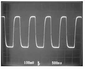
FIG. 1 Probe overcompensation
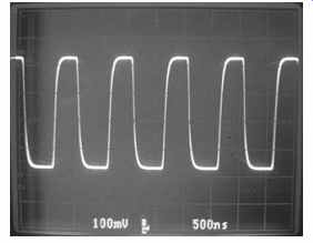
FIG. 2 Probe undercompensation
Vertical Input Attenuator or Volts/Div
The outer ring of this control scales the vertical size of the incoming signal so it will fit on the screen. The voltage marking on each range refers to how many volts it will take to move the trace up or down one division, or box, on the graticule when you're using a 1X probe, which passes the signal straight through to the scope without altering it.
Here's where things get interesting. Remember that 10X/1X switch on the probe? When set to 10X, it divides the incoming signal's voltage by ten. If your probe has no switch, it still does the same thing, as long as it's a 10X probe, which most are. You have to multiply the attenuator's setting by ten to make up for that.
For example, if you measure a voltage that makes the trace rise 3.5 divisions, and your attenuator is set to 0.1 volts/div, multiply 3.5 × 0.1 × 10 to get 3.5 volts.
That might sound overly complicated, but there's an easy way to do it: just move the decimal point one space to the right when looking at the attenuator. If it's set to 0.1 volts/div, remember it's really reading 1 volt/div. Then multiply that by what you see on the screen, and you're all set.
Some fancier scopes automate the 10X factor when used with their own brand of probes. The probes alert the scope to the scaling factor, and the input attenuator's markings are illuminated at the correct spot, so you don't have to do the arithmetic.
When you're interpreting the displayed signal, keep in mind that the precision to which you can measure things depends on the setting of the attenuator. If it's set to 1 volt/div (after accounting for the 10X probe factor, of course), you can visually estimate down to about 0.1 volt using the subdivision lines and the spaces between them. If it's set to 10 volts/div, you can estimate only down to about 1 volt, since the same graticule box now represents 10 volts instead of 1, so each subdivision represents 1 volt.
You may be wondering why probes divide the signal by 10, and why some have switches. To display a signal, the scope has to steal a tiny amount of it from the circuit you're testing. It's like a blood test: you have to take a little blood! The object of the probe's division is to present a very high impedance (essentially, resistance) to the circuit to avoid loading it down-that is, stealing enough current from it to alter its behavior and give you a false representation of its operation. Because the 10X probe needs to steal only a tenth of the signal's actual voltage, it has internal voltage-dividing resistors that give it an impedance of 10 M-ohm, or 10 million ohms. That's very high compared to the resistances used in any common circuit of the sort you'll want to measure. Extremely little current passes through such a high resistance, so the circuit under test doesn't notice it.
If your probe offers 1X, that switch position removes the voltage divider, passing the signal directly to the scope and resulting in an input impedance of 1 M-ohm. That's still pretty high, but it can affect some small-signal and high-frequency circuits.
Usually, you'll keep your probe at 10X unless the signal you want to see is so small that you can't get enough vertical deflection on the screen even with the attenuator set to its most sensitive range. Now and then, you may scope a circuit that generates enough electrical noise to get into the probe through the air, like a radio signal. When you're at 10X, the impedance is so high that it takes very little induced signal to disturb your measurement. Switching to 1X may make the extraneous noise disappear, or at least get much smaller. This kind of thing happens mostly when probing CRT TV sets, LCD backlighting circuits and switching power supplies, all of which use high voltage spikes capable of radiating a significant short-range radio signal.
Using 1X will let you see rather small signals as long as it doesn't load them down too much. Also, some scopes let you pull out the center knob on the attenuator to multiply the sensitivity of the selected range by a factor of 10. Doing so causes some signal degradation, so use this only when you really need it. You probably never will.
Ah, that center knob. It's called the variable attenuator. Normally, you keep it in the fully clockwise, calibrated position so the volts/div you select will match the graticule, allowing you to measure voltage values. Sometimes you want to do a relative measurement-that is, one whose absolute value doesn't matter, but you need to know if it's bigger or smaller than it was before, or its size relative to another signal.
To make such measurements easy to read, it's very helpful to line up both ends of the signal with lines on the graticule. Turning the center knob counterclockwise gradually increases the attenuation, reducing the vertical size of the signal and letting you align its top and bottom with whatever you like. It's crucial to remember, though, that you can't take an actual voltage measurement this way; the vertical spread of the signal has no absolute meaning whenever the variable attenuator is engaged. To remind you, many scopes have a little "uncal" light near the attenuator so you'll know when the variable attenuation is on and the channel is uncalibrated.
Input Coupling (AC/DC/GND)---This determines how the signal is coupled, or transferred, into the vertical amplifiers, and it's one of the most important options on a scope. As you will see, the choice of coupling enables a neat trick for examining signal details and is not limited to being used in the obvious way, with DC for DC signals and AC for AC signals. You'll find yourself switching between the two settings quite often when exploring many types of signals.
GND---The GND setting simply grounds the input of the scope, permitting no voltage or signal from the probe to enter, and discharging the coupling capacitor used in the AC setting. (More about that shortly.) It does not ground the probe tip! You don't need to remove the probe from the circuit under test to switch to the GND setting. This selection is used to position the trace at a desired reference point on the screen, using the input channel's vertical position control, with no influence from incoming signals.
Not all scopes have a GND setting. Some probes offer it on their 10X/1X switches. If you don't have one in either place, it's no big deal, because you can always touch the probe tip to the ground clip. Having a GND setting just makes getting a clean, straight line of 0 volts a bit more convenient.
DC---In the DC position, the signal is directly coupled, and whatever DC voltage is present will be plotted on the screen. If you want to measure the voltage of a power supply or the bias voltage on a transistor, use this position.
To measure a DC voltage, first remove the probe from the circuit and touch it to the ground clip, or switch to the GND setting, and turn the vertical position knob to wherever on the screen you want to call 0 volts. If you're measuring positive voltage, the bottommost graticule line is a good place to put the trace. If the voltage is negative, set the trace at the topmost line, because it will move down when the signal is applied.
Then touch the probe to the point you want to measure, or switch back from GND to DC, and observe how many graticule divisions the trace rises or falls. Don't forget to multiply the attenuator's marking by ten to compensate for your 10X probe! If you touch a voltage point with the probe and the trace disappears, you have probably driven it off the screen with a voltage bigger than can be handled by the range you've selected with the vertical attenuator control, so set that to higher voltages per division until notice the trace. After switching the attenuator to a different range, perform the zero setting again before trying to estimate a measurement from the screen, because sometimes it drifts a little bit when you change the range.
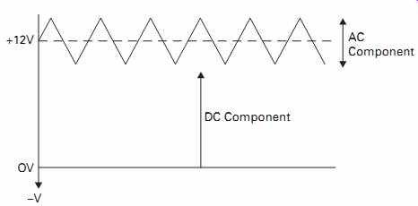
FIG. 3 The AC and DC components of a signal
AC
Many signals contain both DC and AC components. They have a DC voltage offset from 0 volts, but they're also not just a straight line; there's variation in the voltage level, representing information or noise. So how is a varying DC voltage AC? Isn't it one or the other? As I mentioned in Section 5, voltage level and polarity are entirely relative. Any voltage can be positive with respect to one point and negative with respect to another.
Take a look at FIG. 3. That signal is above ground in the positive direction, with none of it going negative, so it's a DC signal with respect to ground, and its height above ground is its DC offset or DC component. The top of it, however, is wiggling up and down. Imagine if you could block the DC offset, and that dotted line became 0 volts. The signal would then be AC, with half above the line and half below.
It looks nice on paper, but you can't actually do that, right? Sure you can! Passing the signal through a capacitor will block the DC level, but, as the signal wiggles, those changes will get through, resulting in a true AC signal swinging above and below ground, with polarity going positive and negative. Hence, those wiggles are known as the AC component of the DC voltage. (And now you know a quick-and-dirty way to turn a positive voltage into a negative one! See, I wasn't kidding, there truly is no absolute polarity.) When you select AC coupling, the scope inserts a coupling capacitor between the probe and the vertical amplifier, blocking any DC voltage from deflecting the beam.
This changes everything! By blocking the DC component of a signal and passing only the AC component, you can examine that component in great detail. Let's see how.
Suppose you have a 12-volt power supply in an LCD monitor with erratic operation. The backlight doesn't like to turn on. When it finally does, sometimes it shuts itself off. You suspect the supply might not be putting out clean power. In other words, some noise could be riding on top of the voltage, perhaps caused by weak filter capacitors, confusing the microprocessor and turning it off. You fire up your scope, set it to DC coupling and check that 12-volt line, but it looks okay. Hmmm…there might be a little blurriness on the line, but it's hard to tell for sure, so you crank up the sensitivity of the vertical attenuator to take a closer look. Oops! The trace is now off the screen. You turn the vertical position control down to get it back, but now that control is as low as it will go. Notice the line, but you can't check for any small spikes or wobbles in it because it keeps going off the screen every time you up the sensitivity enough to examine the small stuff.
If only that same noise were riding on 0 volts, instead of 12, then the trace would stay put and you could fill the screen with even the tiniest changes. No problem.
Switch to AC coupling to block the DC component of the signal and you can crank the attenuator for maximum sensitivity without budging the trace. It's a very powerful technique for examining signals with both DC and AC components. Many signals are of that form, and you'll use AC coupling quite often, regardless of whether the signal is really AC or not. In fact, a true AC signal (one that swings positive and negative with respect to ground, with no DC offset) will read exactly the same with either DC or AC coupling, so switching between the two is an easy way to see if an offset exists.
If the trace doesn't shift vertically when you flip the coupling switch, there's no offset.
If the signal's changes are slow enough, the coupling capacitor charges up and eventually begins to block the slowly changing signal voltage until the other half of the cycle discharges it. This is called low-frequency rolloff; the cap acts as a high pass filter, permitting high frequencies to pass through, while gradually rolling off (attenuating) lower ones, passing nothing when the frequency reaches zero. The effect will distort low-frequency signals, causing their flat areas to droop as the cap charges. See FIG. 4.
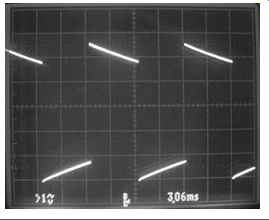
FIG. 4 Tilt due to low-frequency rolloff.
To see this in action, view about four cycles of the square wave from the cal terminal and switch between AC and DC coupling. (Adjust the vertical position if a DC offset moves part of the waveform off the screen when you change the coupling.) The flat tops and bottoms look tilted with AC coupling, losing amplitude and heading toward the middle of the waveform as the cap charges. As the signal frequency rises, the cap has less time to charge, so this effect fades away, for a truer representation of the signal. When you're viewing low-frequency signals with AC coupling, always keep in mind that long, sloping areas may in fact be flat, and the scope's coupling cap might be causing the slope. The easy way to verify the presence of rolloff is to switch to DC coupling (unless a DC offset drives the trace too far off the screen for the vertical position control's range to bring it back). If the sloping lines become flat, you know the cap was fooling you.
After using AC coupling, always ground the probe tip or momentarily switch the input coupler to GND to discharge the coupling capacitor before probing another point. Otherwise, whatever is stored on it will discharge into the next point you touch, confusing your reading and possibly damaging the circuit under test, although there's only a remote chance of that. When you ground the probe, you should see the trace jump for a fraction of a second and then return to where it was as the cap discharges.
AC coupling can be inconvenient when you're working with signals that change amplitude (vertical size) in an asymmetrical fashion. Analog video, for instance, is "clamped" to a fixed voltage, with its sync pulses not deviating from their position at the bottom as the video information at the top changes with the TV picture's content. Using AC coupling with such a signal will cause both ends of the waveform to bounce around as video content rises and falls, because the midpoint of the signal is constantly shifting. The effect is disconcerting and difficult to interpret. Video signals and others with similar asymmetry, like digital pulse streams, are best viewed with DC coupling, so that the unchanging end of the signal stays put.
The example was from a real case of an LCD monitor I fixed using the AC coupling on a DC signal technique. Sure enough, there were narrow, 1/2-volt spikes on the power supply line confusing the microprocessor and tripping the unit off. Once I switched to AC coupling and saw the spikes on the filter capacitor's positive terminal, I didn't even have to check the cap, because I knew a good one would have filtered them out. I just popped in a new cap. A quick check confirmed that the spikes were gone, and the noise on that line was now well under 100 mv. The micro was happy and so was I. The monitor worked great. Without the AC coupling trick, I'd never have known those spikes were there.
Vertical Position---This moves the trace up and down. Use it to set the zero reference point when taking DC measurements. Otherwise, set it wherever is best for examining the signal you're viewing. When using the scope in dual-trace mode, set the two input channels' vertical position controls to keep the waveforms separated. It's conventional to put channel one in the top half of the screen and channel two in the bottom, but you can place them wherever you want, even on top of each other.
Bandwidth Limit---This limits the frequency response of the vertical amplifiers. In 100-MHz scopes, the limit is usually 20 MHz. Switching in the limit removes noise bleeding in from external sources, particularly FM radio stations. With 100-MHz bandwidth, the scope can pick up the lower two-thirds of the FM band, resulting in a noisy-looking signal if you happen to live near an FM broadcast station. Some other radio services may get into your measurements too, if they're strong enough. Leave the bandwidth limit turned off unless noise problems are making your trace blurry.
Vertical Mode--On a dual-trace scope, this selects which channels you will view, and how. Most scopes offer these options:
Ch 1 • You will see only channel 1. Input from channel 2 can still be used to feed the trigger if you want, even though you can't see it.
Ch 2 • The same, but in reverse. You'll see only channel 2.
Add • The voltages of the two channels will be added together and shown as one trace.
Adding two signals together is pretty pointless, so why is this here? One or more of your channels should have a button marked invert or inv. Pressing it makes the channel flip the waveform passing through it upside down, with positive voltages deflecting downward and negative ones upward. If you flip one channel upside down and then select the add mode, the signals will be subtracted, and that is very useful in certain circumstances.
Let's say you have an audio amplifier with some distortion. Or, perhaps, the high frequency response is poor. You want to find which stages are causing the problem.
Feed some audio to the amplifier's input. Set both scope channels to AC coupling.
Connect one channel to a stage's input and the other to the stage's output. If the amplifier hasn't already inverted the signal, do the invert-add trick. Then use the vertical attenuator of the channel with the bigger signal (usually the stage's output) to reduce its displayed amplitude until the signals cancel out and the resulting trace is as flat as possible. What's left is the difference between the two signals: the distortion.
Using this technique, you can easily see what a circuit is doing to a signal, and the results may be enlightening, leading you to a diagnosis. Most amplifier stages will show some difference, but it should be minor. When you see something significant, you've found the errant stage.
Chop--This puts the scope into dual-trace mode, displaying two signals at once.
The two will appear to be independent, and you can set the vertical attenuation and position of each channel at will. The horizontal sweep speed set with the time/div control will apply to both channels, and the scope will trigger and start the sweep based on the timing of whichever of the two channels you choose for triggering.
However, the scope is not truly displaying two simultaneous events; it just looks that way. In reality, it’s rapidly switching between the two channels, with the beam bouncing between them, drawing a little bit of one channel and then a little bit of the other. It’s chopping them up.
This method works very well, ensuring that the time relationship between the two signals is well preserved, since they are really being made by the same beam as it traverses the screen from left to right. It has a few serious limitations, however.
If you crank the sweep speed way up, notice the alternating segments of the two channels and the gaps between them. So, chop mode is not useful at high sweep speeds. Also, if the two signals are harmonically unrelated (their frequencies are not a simple ratio, so the cycles don't coincide), only the channel chosen for triggering will be visible; the other will be a blur.
Alternate or Alt--This is the other dual-trace mode, and it works rather differently.
Instead of chopping the waveform, it draws an entire channel and then goes back and draws the other one, in two separate, alternating sweeps. Alt mode leaves no gaps in the traces, so it's suitable even for very fast sweep speeds. Plus, under certain circumstances, you can view harmonically unrelated signals, with separate triggering for each channel making them both look stable.
Alt mode has its own limitations, though. At slow sweep speeds, you'll see the two sweeps occur, one after the other, with the previous one fading away, resulting in a rather uncomfortable blinking or flashing effect. Also-and this one is much more serious-the timing relationship between the two signals may be disturbed, because of when the scope triggers and how long it takes to sweep the screen before it has a chance to draw the second waveform. In alt mode, the displayed alignment in time of one channel to the other cannot be trusted. Always choose chop mode when you need to compare or align the timing of two signals. In fact, use chop mode as much as possible, and select alt mode only when chopping interferes with the waveform or the two signals you're viewing are unrelated in time, so each one needs its own trigger.
X-Y --- This mode stops the sweep and lets you drive the horizontal deflection from a signal input to channel 2. Be careful when pressing this button, because the stopped beam will create a very bright spot on the screen and can quickly burn the tube's phosphors. Turn the brightness all the way down before trying it, and then gradually turn it up until you see the spot.
At one time, X-Y mode was a useful way of detecting nonlinearity, measuring frequency and some other parameters. Today, it has little or no application, at least not for general service work. I have never needed to use X-Y mode even a single time.
Trigger Controls
To present a stable waveform, the scope must trigger, or begin each sweep, at the same point in each cycle of the incoming signal, so the beam will draw the same signal features on top of the last ones. Otherwise, all you'll see is a blur. Stable triggering is one of the most critical features on a scope, and it's important that you get good at using the trigger controls to achieve it.
Trigger Lock Light---This indicator tells you when the trigger is locked to a feature of the signal. When it's on, you should see a stable waveform. If not, some other control is improperly set, or the trigger may be locking to more than one spot in each cycle of the waveform.
Source --- This selects which channel will be used to trigger the sweep, along with some other options:
Ch 1 • Channel 1's signal will feed the trigger. Use this mode for single-channel operation or for dual-channel work when you want channel 1's signal to control timing.
Ch 2 • Channel 2's signal will feed the trigger.
Alt • In alt mode, each channel will feed the trigger, one after another. This completely invalidates the timing relationship between displayed signals, because you have no idea how much time has elapsed between when the first channel's sweep finished and when the second channel's sweep began. It's useful when you want to look at two signals whose periods are not related, and you want them both to display stably. Just remember that it's like having two separate scopes; no time relationship exists between the displayed signals.
Line • This uses the 60-Hz AC line as a timing reference, generating 60 sweeps per second. It's useful when viewing signals at or very near that frequency whose own features make for difficult triggering. Now and then, it can be handy when troubleshooting line-operated gear, especially linear power supplies.
External or ext • Many scopes have extra inputs that can be used as vertical channels and/or trigger inputs. External triggering is great for locking very complex signals the normal trigger can't get a grip on.
For instance, when adjusting VCR tape paths while viewing the RF (radio-frequency) waveform from the video heads, there is no stable way to trigger at the start of each head's sweep across the tape, using the signal it produces. Instead, you must drive the scope trigger from another signal in the VCR that is synced to the headwheel rotation. The external trigger input provides a place to feed it in, keeping channel 2 (from which you could accomplish the same thing) free for viewing other signals.
Coupling---This is somewhat like the input coupling on the vertical amplifiers, but it offers a few more choices specific to triggering needs:
DC • The trigger will lock to a specific signal voltage relative to ground. It's most useful with asymmetrical waveforms.
AC • The trigger will lock to a voltage above or below the midpoint of the signal, regardless of its voltage relative to ground. It works just like the AC coupling option on the vertical amplifiers, placing a coupling capacitor in line to block the signal's DC component. You can use AC trigger coupling even when you use DC coupling for the vertical channel. Most of the time, you'll use this mode because it makes triggering easy as you look at various signals with different DC components.
HF reject • This feeds the signal through a low-pass filter, smoothing out high frequency noise or signal features that might confuse the trigger and cause it to trip where you don't want it to. If your waveform has high-frequency components causing jittery display, try this option. If you want to trigger on a high-frequency feature, however, selecting HF reject will prevent triggering. Using this setting affects only the trigger operation; the signal going to the vertical amplifier is not filtered.
LF reject • This feeds the signal through a high-pass filter, rolling off low frequencies and preventing them from tripping the trigger. Use it to help trigger on high frequency signal components when lower-frequency elements are causing triggering where you don't want it. Again, the filtering affects only the trigger.
TV-H • This is a specialized trigger mode for use with analog TV signals. It comes from a time when much service work was on TV sets, and not all scopes offer it. It’s optimized to help the scope trigger on the horizontal sync pulses in the TV signal.
TV-V • This enables triggering on the vertical sync pulses in a TV signal.
Slope---This selects whether the trigger locks on signal features that are rising or falling. With many kinds of signals, like audio and oscillators, it doesn't matter.
Normally, leave it on +. When you want to trigger on the falling edge of a waveform, switch it to -. To see the slope feature in action, connect the probe to the cal terminal, get a locked waveform and then switch between the slopes. Look at the leftmost edge of the screen to see what the waveform was doing when the sweep triggered.
Level---This sets the voltage level at which the trigger will trip. It has no calibration.
Just turn it back and forth until the trigger locks. If the trigger stays locked through a wide swath of this control's range, that indicates a solid trigger lock, and you should see a very stable display. If you can get trigger lock only over a very narrow range of the level control, the lock is not great, and you can expect the waveform to jump around if the signal level or shape changes even a little bit. To get a better grip on the signal, try the various coupling options, especially HF reject and LF reject, rotating the level control back and forth for each one.
Holdoff---This keeps the trigger held off, or unable to trip, for an adjustable period of time after its last trigger event. It's used on complex signals with irregularly spaced features of similar voltages, to avoid having more than one in each cycle trip the trigger and blur the displayed waveform. If you can't get a waveform to stabilize any other way, try turning this control. Otherwise, keep it at the "normal" position, which reduces holdoff to a minimum. Forgetting and leaving it on can make triggering confusingly difficult, as the holdoff will make the trigger miss consecutive cycles if it's set for too long a period, resulting in a jumpy mess.
Horizontal Controls
The horizontal axis represents time, and the scope's drawing of the waveform from left to right is called the sweep. The settings controlling it determine what you'll see, even more than do those for the vertical parameters.
Horizontal Position---This positions the trace left and right. Set it to fill the screen, with the left edge of the trace just off the left side. Now and then you may wish to line up a signal feature with the graticule to make a rough measurement of period or frequency, and you can use this control to do so.
Sweep Mode --This control offers three options: auto, normal and single.
Auto • The trigger will lock to the incoming signal, and sweep will begin. When there's no signal, or the trigger isn't locking on it for some reason, the sweep will go into free-run mode, triggering itself continuously so notice a flat line, or, in the case of trigger unlock, a blur. This is the mode you will use most of the time.
Normal • Sweep will begin when the trigger locks on a signal but will stop when the signal ceases. This can be handy for observing when rapid interruptions occur in intermittent signals, because the trace will blink at the moment the signal disappears. It's a little disconcerting sometimes, though, because if the screen goes blank, you don't know why. Maybe the trace is off the screen, maybe the brightness is too low, or maybe the trigger isn't locked.
Single • This is for single-sweep mode, in which the trigger will initiate one sweep and then halt until you press the reset button (which may be the single button itself). It helps you determine when a signal has occurred, because you'll see the flash of one sweep go by. Look for a little indicator light near the single button labeled Ready or Armed. When it's lit, the sweep can be fired one time.
After that firing, the light will go out, and you must press the reset button to rearm the sweep. You won't use this mode very often.
Time/Div---The outer ring of this large control sets the timebase, or sweep speed at which the beam will travel across the screen from left to right. It’s calibrated by time in seconds, milliseconds (ms, or thousandths of a second) and microseconds (µs, or millionths of a second). The calibration number refers to how long the beam will take to traverse one division, or graticule box.
For a signal of a given frequency, the faster you set the sweep, the more horizontally spread the display will be, and the fewer cycles of the signal you will see at one time.
Often, you will want to set it as fast as possible to see the most detail, but not always.
In some instances, the aggregate effect of many displayed signal cycles can be more revealing than is a singular signal feature. If you have low-frequency variation, such as AC line hum, on a fairly fast signal, you can't see the hum if the sweep is set fast enough to see individual cycles of the signal. But when you turn the sweep speed low enough to view a 60-cycle event, you will see the hum clearly, even though the signal itself will be too crammed together to be resolvable.
To see the effects of various sweep rates, look at the calibrator's square wave and click the time/div knob through its ranges. On most scopes, the number of displayed waves will grow or shrink with the sweep rate. If it doesn't, your scope is changing the frequency of the calibrator to match the timebase. Some of them do that.
Variable Time---The center knob uncalibrates the timebase, slowing it down as you turn the knob counterclockwise. This is the horizontal equivalent of the vertical channels' variable attenuators, and it can be useful for lining events up with the graticule during relative time measurements of two signals. Normally, you'll leave it in the fully clockwise position. As with the variable attenuators, it has an "uncal" light to remind you that the timebase no longer matches the graticule.
Pull X10---On most scopes, pulling out the variable time knob speeds up the sweep rate by a factor of ten. The sweep does remain calibrated in this mode. It's a quick and-dirty way to spread out a signal, and it also lets you get to the very fastest sweep rate by turning the time/div knob all the way up and then pulling this one out.
Normally, keep this knob pushed in, and pull it only when you really need it. Don't forget to push it in again, or your time measurements will be off by a factor of ten.
Delayed Sweep Controls
Delayed sweep is an advanced scope function you won't need for basic repair work, but it's worth learning for those more complex situations, like servicing camcorder motor control servos, in which it's essential. My apologies for any neck injuries caused by making your head spin while reading this section! Once you actually play with delayed sweep a few times, you'll discover it's really not difficult, and it's quite nifty.
With delayed sweep, your scope becomes a magnifying glass, allowing you to zoom in on any signal feature, even though it's not the one on which you're triggering the main sweep. Why do this? It's very powerful, providing a level of signal detail you couldn't otherwise examine.
Let's say you have a sine wave from an oscillator, but it doesn't look quite right.
A spike or something is distorting its shape at a particular spot. It's hard to tell what it is, but notice a thickening of the trace at that point. You want to get up close and personal with that spot so you can really see the details of the distortion and determine what's causing it. You scope the sine wave and crank up the sweep rate, but when you get it going fast enough to spread out the mystery spot, it has already gone off the right side of the screen. You turn the sweep rate down a little bit, but now the signal is too crammed together to permit a good look at the spot.
Cue superhero music. This is a job for…Delayed Sweep, Slayer of Stubborn Signals, Vanquisher of Villainous Voltages! In this mode, the scope triggers on the waveform as usual, as set by the A trigger. It begins sweeping at the rate selected with the main time/div knob. After a period of time you set with the delay time multiplier knob, the B timebase takes over and the beam finishes the sweep at the speed set by that timebase's knob, the one inside the main sweep's knob.
The result is a compound view of the signal, with a lower sweep rate for the events leading up to your spot of interest, followed by a stretched-out, detailed view of the spot! Even cooler, you can rotate the delay time multiplier knob and scan through the entire signal, examining any part of it. It's practically a CAT scan for circuitry, and you don't even need a litter box. Let's look at the controls involved with setting up the delayed sweep mode.
Delay Time or B Timebase
This control, located inside the main time/div knob, sets the speed of the B sweep, which stretches out the waveform for close examination.
Think of it like a zoom lens on a camera: the faster you set it, the more you're zooming in for a closer look at a smaller area.
On some scopes, notably those made by Tektronix, the same knob is used for both the A and B sweeps. To engage the B sweep, you pull out the knob, mechanically separating the two timebase controls. In this position, the outer ring, which sets the A sweep rate, won’t move when you turn the knob clockwise to speed up the B sweep.
Horizontal Display Mode
This selects which timebase (sweep generator) will drive the beam across the screen, and is how you choose between normal and delayed sweep modes.
A • The main timebase, which is set by the big time/div control, will control the sweep. Delayed sweep mode won’t be engaged.
B • The secondary timebase, set by the smaller control inside the time/div knob, will control the sweep. This may be set equal to or faster than the main timebase, but not slower.
Alt • Both timebases will be displayed, one on top of the other. The A sweep's display will be highlighted over the area that the B sweep is stretching out. The faster you make the B sweep rate, the narrower the highlight will get, and the more stretched the displayed B sweep will be. See FIG. 5. Look for a knob called trace separation. It lets you position the B sweep's display above or below that of the A sweep, so notice them better. It has no calibration or meaning in voltage measurement terms; it's just a convenience.
If your scope has two brightness controls, you may need to increase the brightness of the B sweep to keep it visible at high sweep rates. The faster the beam sweeps, the dimmer it will appear.
A intens B • This stands for "A intensified by B" and shows you the A sweep and the highlight of the portion of the signal the B sweep will cover, just as is shown in Alt mode. It's useful for zeroing in on the spot you wish to examine without cluttering up the screen with the B trace, before you switch to a mode that displays B.
In both Alt and A intens B modes, the highlighting of the A sweep may not be visible if you have the A brightness control set too high. Try turning it down for a more prominent highlight.
===
FIG. 5 Alt mode delayed sweep display of the rising edge of the scope's calibrator square wave. The A trace is on the top, with the B trace below it. Notice the highlighting of the portion of the waveform being stretched out by the B trace.
Highlighted area Magnified view of highlighted area using B sweep A sweep
===
B • This shows only the B trace, at the sweep rate selected by the B or delay time setting (the knob inside the big, outer time/div one). It turns off the A trace, but the settings which result in the delayed sweep B view remain in effect, including triggering, A sweep rate and delay time. Once you've zoomed in on your spot of interest, you can switch to this setting to see only the detailed area, without the main waveform from which it’s derived. In this mode, the trace separation control doesn't do anything.
Start after delay/triggered • This determines what happens after the A sweep has reached the beginning of the intensified area where it will switch to B. In start after delay mode, the B sweep begins as soon as the A sweep hits that point.
This lets you scan continuously through the signal with the delay time multiplier control, and is my preferred way of using delayed sweep. It has one drawback, though. Any jitter (instability) in the triggering of the A sweep will get magnified by the faster sweep rate of the B sweep, resulting in the stretched waveform's wobbling back and forth. Sometimes the wobble is bad enough to make examining the signal difficult.
To remove the wobble, select the start triggered mode. Then, when the A sweep reaches the intensified portion, the B sweep will wait for a trigger before beginning. This is what those B trigger controls are for. What's great about having a separate trigger for this function is that you don't have to use the same trigger settings for the B sweep that you selected for the main trigger. So, you can treat the detailed area as a separate signal, setting the trigger for best operation on its particular features.
The downside to this mode is that you cannot scroll smoothly through a signal, because the B sweep waits for a trigger. Notice only features on which it has triggered. Keep your scope in start after delay mode unless you run into wobble problems or are examining fine details in a complex signal, like an analog video signal, with many subparts.
Delay Time Multiplier
This sets how many horizontal divisions the delay will wait before starting the B sweep (or looking for a new trigger for it, in the start triggered mode), and is referenced to the A sweep rate. For example, if the A sweep is set to 0.1 ms and the delay time multiplier knob is at 4.5, it'll wait 0.45 ms before the highlighted area begins. For most work, you can ignore the numbers and just keep turning the knob to scan through the signal, using the highlight to pick your expansion area. Most scopes provide a vernier (gear reduction) knob for fine control.
B Ends A
This turns off the A sweep after the B sweep starts. On some scopes, it presents both sweeps in one line, switching from A to B when B begins. On others, the two sweeps are still on separate lines, and A just disappears after the point where B takes over.
Try It!
How are those neck muscles doing? Ready to try some of this? Let's use delayed sweep to get a close-up look at the rising edge of your scope's calibrator square wave.
Connect the probe to the cal terminal and set up the scope for normal, undelayed operation by selecting the A horizontal display mode. Adjust the vertical, trigger and time/div controls to see a couple of cycles on the screen, and put them on the top half.
Disengage B ends A mode if it’s currently turned on. Make sure start after delay is engaged, not start triggered. Select the A intens B mode and move the delay time multiplier knob to center the highlight over the leading (rising) edge of the square wave, with the start of the highlight just before (to the left of) the edge. Set the brightness controls as desired so notice the highlight clearly. The A brightness control will adjust the bulk of the waveform, with the B brightness setting the highlight's intensity.
If more than one cycle of the waveform is on the screen, any of the leading edges will do. It's best to keep the A sweep as fast as possible, though, without losing the feature you want to examine off the right side, so try not to have more than one or two cycles visible.
Adjust the delay time (B sweep rate) so that the highlight is just a little wider than the edge, covering a smidge of the waveform before and after it. Note that the faster you make the B sweep, the narrower the highlight gets, meaning you will be zooming in on a smaller area, enlarging it proportionally more.
Now switch to alt mode. You should see the zoomed-in rising edge of the waveform superimposed on the original wave. Use the trace separator knob to move it down so notice it clearly. Increase the B sweep rate one step at a time. As you crank it up, the magnified edge will move off the right side of the screen, and you'll have to turn the delay time multiplier knob clockwise just a tad to bring it back. If the magnified waveform gets too dim, crank up the B brightness.
When you get the B sweep going pretty fast, you can clearly see the edge's slope, and you may also notice some wobbles or other minuscule features at its bottom and top, details you can't see at all without the magic of delayed sweep! For fun, scan through the waveform with the delay time multiplier knob, and take a look at the falling edge too. Pretty awesome, isn't it? Enjoy! Just don't forget to turn the A brightness down when you switch back to normal, undelayed operation, if you turned it up.
FIG. 6 Cursors and frequency (1/time) measurement on a Tektronix 2445
analog scope
Cursor Controls
If your scope offers numerical calculation, it will have cursor controls that let you specify the parts of the waveform you wish to measure. The results of the measurements will be shown as numbers on the screen, along with the waveforms.
The layout of controls can vary quite a bit in this department, but the principles are pretty universal. For amplitude measurements, you move two horizontal cursors up and down to read the voltage difference between them. For time measurements, you move two vertical cursors left and right to measure the time difference between them, or to calculate approximate frequency. See FIG. 6.
On some scopes, you can lock one cursor to the other after you've set them, so you can move one to the start of a waveform feature and the other will follow, letting you see how the signal aligns against the second one.
Always keep in mind that these measurements provide nowhere near the accuracy or precision of those you'll get from your DMM or frequency counter! Still, you can't measure the voltage or frequency of items within signals with anything but a scope.
Digital Differences
Operating a digital scope isn't that much different from using an analog, but there are some items to keep in mind.
First, many of the controls on an analog instrument are replaced by menus on its digital counterpart. This approach unclutters the front panel, but it's slower and more awkward to have to step through nested menus than it’s to reach for a knob. As long as you keep the basic functions of vertical, horizontal and triggering in mind, though, you should have no trouble remembering where to find the options you need.
All the screen controls are gone. You don't need astigmatism, focus, illumination and separate A and B brightness, because the display is an LCD screen and it’s not being swept at varying rates by a beam. You'll find a main brightness or contrast adjustment in a menu. Once set, it won't require any changes for different modes or sweep speeds.
The display will show various operating parameters like trigger status, volts/div and time/div, so you don't have to take your eyes off the screen and interpret a bunch of controls.
Digitals are generally more accurate, especially in the horizontal (time) domain.
They also tend to have more stable triggering and very little drift.
Delayed sweep may be handled a bit differently. On the Tektronix TDS-220, for instance, the equivalent of the analog scope's highlight is called the Window Zone, and you set the delay time multiplier and window width using the horizontal position and time knobs after selecting the mode from a menu. Instead of a highlight, you get a set of long, vertical cursors. Then you select Window to see the magnified waveform. The principles are the same, of course, but there's no equivalent to the analog instrument's alt mode, in which both the undelayed and delayed sweeps are shown simultaneously.
More than likely, the digital scope will include various acquisition modes, so you can grab waveforms, store them and display them along with live signals. It'll probably also have measurement options for frequency, period, peak-to-peak voltage, RMS voltage and so on. Especially nice is the auto setup function, which sets the vertical, horizontal and trigger for proper display of a cycle or two of most waveforms, without your having to twist a single knob. Hook up the probe, hit the auto button and there's your signal. It's the oscilloscope equivalent of autoranging on a DMM, and it saves you a lot of time and effort.
Reading the screen on a digital scope requires more interpretation. The limitations imposed by the digital sampling process, the finite resolution of the dot-matrix display and the slower-than-real-time screen updating have to be kept in mind at all times. For one thing, curved areas can have jagged edges, and it's important to remember that they are not really in the signal. Also, lines may appear thicker and noisier than they really are, due to digital sampling noise. Aliasing of the signal against the sampling rate and also against the screen resolution can seriously misrepresent waveforms under certain circumstances, as discussed in Section 2. Finally, the slow updating means some details get missed. All scopes, analog or digital, show you snapshots, but with digitals there's much more time between snaps.
When the input signal disappears, many digital scopes freeze the waveform on the screen for a moment before the auto sweep kicks in and replaces it with a flat line.
This makes it hard to know exactly when signals stop. If you're wiggling a board while watching for an intermittent, the time lag can hinder your efforts to locate the source of the dropout.
Overall, a digital instrument offers more stability, options and conveniences, but an analog scope gives you a truer representation. As with just about everything, digital is the future, like it or not, and analog scopes will probably disappear from the marketplace in the next few years. If you snagged a good one, hang onto it! If you chose a digital instrument, just keep these caveats in mind and you'll be fine.