AMAZON multi-meters discounts AMAZON oscilloscope discounts
OUTLINE
- 1. Basic Filter Responses
- 2. Filter Response Characteristics
- 3. Active Low-Pass Filters
- 4. Active High-Pass Filters
- 5. Active Band-Pass Filters
- 6. Active Band-Stop Filters
- 7. Filter Response Measurements
- Application Activity
- Programmable Analog Technology
OBJECTIVES:
-- Describe and analyze the gain-versus-frequency responses of basic types of filters
-- Describe three types of filter response characteristics and other parameters
-- Identify and analyze active low-pass filters
-- Identify and analyze active high-pass filters
-- Analyze basic types of active band-pass filters
-- Describe basic types of active band-stop filters
-- Discuss two methods for measuring frequency response
TERMINOLOGY
-- Filter
-- Low-pass filter
-- Pole
-- Roll-off
-- High-pass filter
-- Band-pass filter
-- Band-stop filter
-- Damping factor
APPLICATION ACTIVITY PREVIEW
RFID stands for Radio Frequency Identification and is a technology that enables the tracking and/or identification of objects. Typically, an RFID system consists of an RF tag containing an IC chip that transmits data about the object, a reader that receives transmitted data from the tag, and a data-processing system that processes and stores the data passed to it by the reader. In this application, you will focus on the RFID reader. RFID systems are used in metering applications such as electronic toll collection, inventory control and tracking, merchandise control, asset tracking and recovery, tracking parts moving through a manufacturing process, and tracking goods in a supply chain.
INTRODUCTION
Power supply filters were introduced in section 2. In this section, active filters that are used for signal processing are introduced. Filters are circuits that are capable of passing signals with certain selected frequencies while rejecting signals with other frequencies. This property is called selectivity.
Active filters use transistors or op-amps combined with passive RC, RL, or RLC circuits. The active devices provide voltage gain, and the passive circuits provide frequency selectivity. In terms of general response, the four basic categories of active filters are low-pass, high-pass, band-pass, and band stop. In this section, you will study active filters using op amps and RC circuits.
+++++++++++++++++++++++++
1. BASIC FILTER RESPONSES
Filters are usually categorized by the manner in which the output voltage varies with the frequency of the input voltage. The categories of active filters are low-pass, high pass, band-pass, and band-stop. Each of these general responses are examined.
After completing this section, you should be able to:
-- Describe and analyze the gain-versus-frequency responses of basic types of filters
-- Describe low-pass filter response
-- Define passband and critical frequency
-- Determine the bandwidth
-- Define pole
-- Explain roll-off rate and define its unit
-- Calculate the critical frequency
-- Describe high-pass filter response
-- Explain how the passband is limited
-- Calculate the critical frequency
-- Describe band-pass filter response
-- Determine the bandwidth
-- Determine the center frequency
-- Calculate the quality factor (Q)
-- Describe band-stop filter response
-- Determine the bandwidth
Low-Pass Filter Response
A filter is a circuit that passes certain frequencies and attenuates or rejects all other frequencies. The passband of a filter is the range of frequencies that are allowed to pass through the filter with minimum attenuation (usually defined as less than -3dB of attenuation). The critical frequency, (also called the cutoff frequency) fc defines the end of the passband and is normally specified at the point where the response drops -3dB (70.7%) from the passband response. Following the passband is a region called the transition region that leads into a region called the stopband. There is no precise point between the transition region and the stopband.
A low-pass filter is one that passes frequencies from dc to fc and significantly attenuates all other frequencies. The passband of the ideal low-pass filter is shown in the blue shaded area of FIG. 1(a); the response drops to zero at frequencies beyond the pass band. This ideal response is sometimes referred to as a "brick-wall" because nothing gets through beyond the wall. The bandwidth of an ideal low-pass filter is equal to fc.
BW=fc (Equation 1)
The ideal response shown in FIG. 1(a) is not attainable by any practical filter. Actual filter responses depend on the number of poles, a term used with filters to describe the number of RC circuits contained in the filter. The most basic low-pass filter is a simple RC circuit consisting of just one resistor and one capacitor; the output is taken across the capacitor as shown in FIG. 1(b). This basic RC filter has a single pole, and it rolls off at -20 dB/decade beyond the critical frequency. The actual response is indicated by the blue line in FIG. 1(a). The response is plotted on a standard log plot that is used for filters to show details of the curve as the gain drops. Notice that the gain drops off slowly until the frequency is at the critical frequency; after this, the gain drops rapidly.
The -20 dB/decade roll-off rate for the gain of a basic RC filter means that at a frequency of 10fc the output will be -20 dB (10%) of the input. This roll-off rate is not a particularly good filter characteristic because too much of the unwanted frequencies (beyond the passband) are allowed through the filter.
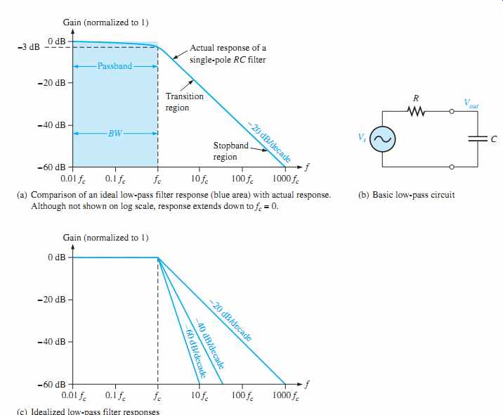
FIG. 1 Low-pass filter responses.
(a) Comparison of an ideal low-pass filter response (blue area) with actual response.
Although not shown on log scale, response extends down to fc = 0.
(b) Basic low-pass circuit
The critical frequency of a low-pass RC filter occurs when XC = R, where
fc =1/[2 pi RC]
Recall from your basic dc/ac studies that the output at the critical frequency is 70.7% of the input. This response is equivalent to an attenuation of -3 dB.
FIG. 1(c) illustrates three idealized low-pass response curves including the basic one-pole response (-20 dB/decade). The approximations show a flat response to the cut off frequency and a roll-off at a constant rate after the cutoff frequency. Actual filters do not have a perfectly flat response up to the cutoff frequency but drop to -3dB at this point as described previously.
In order to produce a filter that has a steeper transition region (and hence form a more effective filter), it is necessary to add additional circuitry to the basic filter. Responses that are steeper than -20 dB/decade in the transition region cannot be obtained by simply cascading identical RC stages (due to loading effects). However, by combining an op-amp with frequency-selective feedback circuits, filters can be designed with roll-off rates of -40, -60, or more dB/decade. Filters that include one or more op-amps in the design are called active filters. These filters can optimize the roll-off rate or other attribute (such as phase response) with a particular filter design. In general, the more poles the filter uses, the steeper its transition region will be. The exact response depends on the type of filter and the number of poles.
High-Pass Filter Response
A high-pass filter is one that significantly attenuates or rejects all frequencies below fc and passes all frequencies above fc.The critical frequency is, again, the frequency at which the output is 70.7% of the input (or -3dB) as shown in FIG. 2(a). The ideal response, indicated by the blue-shaded area, has an instantaneous drop at fc which, of course, is not achievable. Ideally, the passband of a high-pass filter is all frequencies above the critical frequency. The high-frequency response of practical circuits is limited by the op-amp or other components that make up the filter.
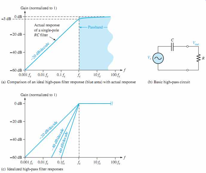
FIG. 2 High-pass filter responses. Comparison of an ideal high-pass filter
response (blue area) with actual response (a) Basic high-pass circuit (b);
(c) Idealized high-pass filter responses
A simple RC circuit consisting of a single resistor and capacitor can be configured as a high-pass filter by taking the output across the resistor as shown in FIG. 2(b). As in the case of the low-pass filter, the basic RC circuit has a roll-off rate of as indicated by the blue line in FIG. 2(a). Also, the critical frequency for the basic high pass filter occurs when XC = R, where
fc = 1/[2 pi RC ]
FIG. 2(c) illustrates three idealized high-pass response curves including the basic one-pole response for a high-pass RC circuit. As in the case of the low pass filter, the approximations show a flat response to the cutoff frequency and a roll-off at (-20 dB/decade) -20 dB/decade, a constant rate after the cutoff frequency. Actual high-pass filters do not have the perfectly flat response indicated or the precise roll-off rate shown. Responses that are steeper than -20 dB/decade in the transition region are also possible with active high-pass filters; the particular response depends on the type of filter and the number of poles.
Band-Pass Filter Response
A band-pass filter passes all signals lying within a band between a lower-frequency limit and an upper-frequency limit and essentially rejects all other frequencies that are outside this specified band. A generalized band-pass response curve is shown in FIG. 3. The bandwidth (BW) is defined as the difference between the upper critical frequency ( fc2) and the lower critical frequency ( fc1).
BW = fc2 - fc1 (Equation 2)
The critical frequencies are, of course, the points at which the response curve is 70.7% of its maximum. Recall from section 12 that these critical frequencies are also called 3 dB frequencies. The frequency about which the passband is centered is called the center frequency, f0, defined as the geometric mean of the critical frequencies.
f0 = √ (fc1 fc2) [ Equation 3]
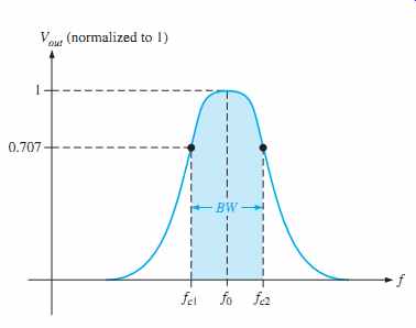
FIG. 3 General band-pass response curve.
Quality Factor The quality factor (Q) of a band-pass filter is the ratio of the center frequency to the bandwidth.
Q = f0/BW ( Equation 4)
The value of Q is an indication of the selectivity of a band-pass filter. The higher the value of Q, the narrower the bandwidth and the better the selectivity for a given value of f0. Band-pass filters are sometimes classified as narrow-band (Q > 10) or wide-band (Q < 10). The quality factor (Q) can also be expressed in terms of the damping factor (DF) of the filter as:
Q = 1/DF
You will study the damping factor in Section 2.
Band-Stop Filter Response
Another category of active filter is the band-stop filter, also known as notch, band-reject, or band-elimination filter. You can think of the operation as opposite to that of the band pass filter because frequencies within a certain bandwidth are rejected, and frequencies outside the bandwidth are passed. A general response curve for a band-stop filter is shown in FIG. 4. Notice that the bandwidth is the band of frequencies between the 3 dB points, just as in the case of the band-pass filter response.
FIG. 4 General band-stop filter response.
SECTION 1 CHECKUP
1. What determines the bandwidth of a low-pass filter?
2. What limits the passband of an active high-pass filter?
3. How are the Q and the bandwidth of a band-pass filter related? Explain how the selectivity is affected by the Q of a filter.
-------------------
2. FILTER RESPONSE CHARACTERISTICS
Each type of filter response (low-pass, high-pass, band-pass, or band-stop) can be tailored by circuit component values to have either a Butterworth, Chebyshev, or Bessel characteristic. Each of these characteristics is identified by the shape of the response curve, and each has an advantage in certain applications.
After completing this section, you should be able to:
-- Describe three types of filter response characteristics and other parameters
-- Discuss the Butterworth characteristic
-- Describe the Chebyshev characteristic
-- Discuss the Bessel characteristic
-- Define damping factor
-- Calculate the damping factor
-- Show the block diagram of an active filter
-- Analyze a filter for critical frequency and roll-off rate
-- Explain how to obtain multi-order filters
-- Describe the effects of cascading on roll-off rate
Butterworth, Chebyshev, or Bessel response characteristics can be realized with most active filter circuit configurations by proper selection of certain component values. A general comparison of the three response characteristics for a low-pass filter response curve is shown in FIG. 5. High-pass and band-pass filters can also be designed to have any one of the characteristics.
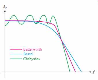
FIG. 5 Comparative plots of three types of filter response characteristics.
The Butterworth Characteristic
The Butterworth characteristic provides a very flat amplitude response in the passband and a roll-off rate of -20 dB/decade/pole.
The phase response is not linear, however, and the phase shift (thus, time delay) of signals passing through the filter varies nonlinearly with frequency. Therefore, a pulse applied to a filter with a Butterworth response will cause overshoots on the output because each frequency component of the pulse's rising and falling edges experiences a different time delay. Filters with the Butterworth response are normally used when all frequencies in the passband must have the same gain. The Butterworth response is often referred to as a maximally flat response.
The Chebyshev Characteristic
Filters with the Chebyshev response characteristic are useful when a rapid roll-off is required because it provides a roll-off rate greater than -20 dB/decade/pole. This is a greater rate than that of the Butterworth, so filters can be implemented with the Chebyshev response with fewer poles and less complex circuitry for a given roll-off rate. This type of filter response is characterized by overshoot or ripples in the passband (depending on the number of poles) and an even less linear phase response than the Butterworth.
The Bessel Characteristic
The Bessel response exhibits a linear phase characteristic, meaning that the phase shift increases linearly with frequency. The result is almost no overshoot on the output with a pulse input. For this reason, filters with the Bessel response are used for filtering pulse waveforms without distorting the shape of the waveform.
The Damping Factor
As mentioned, an active filter can be designed to have either a Butterworth, Chebyshev, or Bessel response characteristic regardless of whether it is a low-pass, high-pass, band-pass, or band-stop type. The damping factor (DF ) of an active filter circuit determines which response characteristic the filter exhibits. To explain the basic concept, a generalized active filter is shown in FIG. 6. It includes an amplifier, a negative feedback circuit, and a filter section. The amplifier and feedback are connected in a noninverting configuration.
The damping factor is determined by the negative feedback circuit and is defined by the following equation:
DF = 2 - R1 / R2 [Equation 5 ]
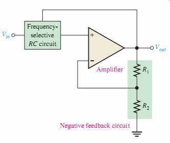
FIG. 6 General diagram of an active filter.
Basically, the damping factor affects the filter response by negative feedback action.
Any attempted increase or decrease in the output voltage is offset by the opposing effect of the negative feedback. This tends to make the response curve flat in the passband of the filter if the value for the damping factor is precisely set. By advanced mathematics, which we will not cover, values for the damping factor have been derived for various orders of filters to achieve the maximally flat response of the Butterworth characteristic.
The value of the damping factor required to produce a desired response characteristic depends on the order (number of poles) of the filter. A pole, for our purposes, is simply a circuit with one resistor and one capacitor. The more poles a filter has, the faster its roll-off rate is. To achieve a second-order Butterworth response, for example, the damping factor must be 1.414. To implement this damping factor, the feedback resistor ratio must be
R1/ R2 = 2 - DF = 2 - 1.414 = 0.586
This ratio gives the closed-loop gain of the noninverting amplifier portion of the filter, a value of 1.586, derived as follows:

Critical Frequency and Roll-Off Rate
The critical frequency is determined by the values of the resistors and capacitors in the frequency-selective RC circuit shown in FIG. 6. For a single-pole (first-order) filter, as shown in FIG. 7, the critical frequency is:
fc =1/(2 pi RC)
Although we show a low-pass configuration, the same formula is used for the fc of a single pole high-pass filter. The number of poles determines the roll-off rate of the filter. A Butterworth response produces -20 dB/decade/pole. So, a first-order (one-pole) filter has a roll-off of -20 dB/decade; a second-order (two-pole) filter has a roll-off rate of -40 dB/decade; a third-order (three-pole) filter has a roll-off rate of -60 dB/decade; and so on.
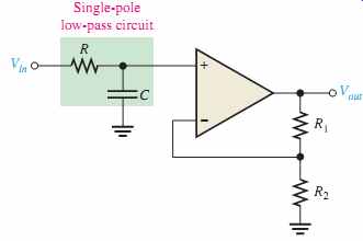
FIG. 7 First-order (one-pole) low-pass filter.
Generally, to obtain a filter with three poles or more, one-pole or two-pole filters are cascaded, as shown in FIG. 8. To obtain a third-order filter, for example, cascade a second-order and a first-order filter; to obtain a fourth-order filter, cascade two second-order filters; and so on. Each filter in a cascaded arrangement is called a stage or section.
Because of its maximally flat response, the Butterworth characteristic is the most widely used. Therefore, we will limit our coverage to the Butterworth response to illustrate basic filter concepts. Table 1 lists the roll-off rates, damping factors, and feed back resistor ratios for up to sixth-order Butterworth filters. Resistor designations correspond to the gain-setting resistors in FIG. 8 and may be different on other circuit diagrams.
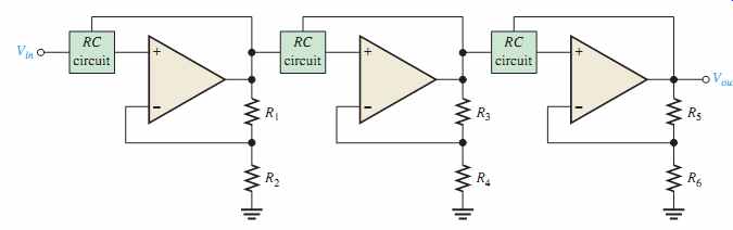
FIG. 8 The number of filter poles can be increased by cascading.
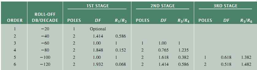
TABLE 1 Values for the Butterworth response.
SECTION 2 CHECKUP
1. Explain how Butterworth, Chebyshev, and Bessel responses differ.
2. What determines the response characteristic of a filter?
3. Name the basic parts of an active filter.
3. ACTIVE LOW-PASS FILTERS
Filters that use op-amps as the active element provide several advantages over passive filters (R, L, and C elements only). The op-amp provides gain, so the signal is not attenuated as it passes through the filter. The high input impedance of the op-amp prevents excessive loading of the driving source, and the low output impedance of the op-amp prevents the filter from being affected by the load that it is driving. Active filters are also easy to adjust over a wide frequency range without altering the desired response.
After completing this section, you should be able to:
-- Identify and analyze active low-pass filters
-- Identify a single-pole low-pass filter circuit
-- Determine the closed-loop voltage gain
-- Determine the critical frequency
-- Identify a Sallen-Key low-pass filter circuit
-- Describe the filter operation
-- Calculate the critical frequency
-- Analyze cascaded low-pass filters
-- Explain how the roll-off rate is affected
A Single-Pole Filter
FIG. 9(a) shows an active filter with a single low-pass RC frequency-selective circuit that provides a roll-off of -20 dB/decade above the critical frequency, as indicated by the response curve in FIG. 9(b). The critical frequency of the single-pole filter is fc = 1/(2 pi RC).
The op-amp in this filter is connected as a noninverting amplifier with the closed-loop voltage gain in the passband set by the values of R1 and R2.
Acl(NI) = R1/R2 = 1 [ Equation 6]
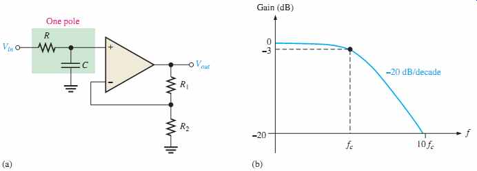
FIG. 9 Single-pole active low-pass filter and response curve.
The Sallen-Key Low-Pass Filter
The Sallen-Key is one of the most common configurations for a second-order (two-pole) filter. It is also known as a VCVS (voltage-controlled voltage source) filter. A low-pass version of the Sallen-Key filter is shown in FIG. 10. Notice that there are two low pass RC circuits that provide a roll-off of -40 dB/decade above the critical frequency (assuming a Butterworth characteristic). One RC circuit consists of RA and CA, and the second circuit consists of CB and RB. A unique feature of the Sallen-Key low-pass filter is the capacitor CA that provides feedback for shaping the response near the edge of the passband. The critical frequency for the Sallen-Key filter is:

Equation 7
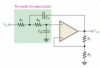
FIG. 10 Basic Sallen-Key low-pass filter.
The component values can be made equal so that RA = RB = R and CA = CB = C . In this case, the expression for the critical frequency simplifies to:
fc = 1/[2 pi RC]
As in the single-pole filter, the op-amp in the second-order Sallen-Key filter acts as a noninverting amplifier with the negative feedback provided by resistors R1 and R2. As you have learned, the damping factor is set by the values of R1 and R2, thus making the filter response either Butterworth, Chebyshev, or Bessel. For example, from Table 1, the R1/R2 ratio must be 0.586 to produce the damping factor of 1.414 required for a second-order Butterworth response.
Cascaded Low-Pass Filters
A three-pole filter is required to get a third-order low-pass response (-60 dB/decade). This is done by cascading a two-pole Sallen-Key low-pass filter and a single-pole low-pass filter, as shown in FIG. 12(a). FIG. 12(b) shows a four-pole configuration obtained by cascading two Sallen-Key (2-pole) low-pass filters. In general, a four-pole filter is preferred because it uses the same number of op-amps to achieve a faster roll-off.
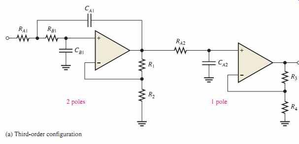
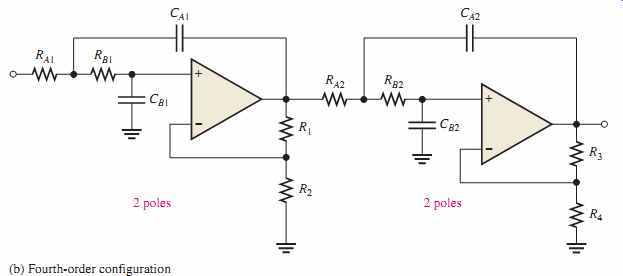
FIG. 12 Cascaded low-pass filters. (a) Third-order configuration; (b)
Fourth-order configuration
SECTION 3 CHECKUP
1. How many poles does a second-order low-pass filter have? How many resistors and how many capacitors are used in the frequency-selective circuit?
2. Why is the damping factor of a filter important?
3. What is the primary purpose of cascading low-pass filters?
4. ACTIVE HIGH-PASS FILTERS
In high-pass filters, the roles of the capacitor and resistor are reversed in the RC circuits.
Otherwise, the basic parameters are the same as for the low-pass filters.
After completing this section, you should be able to:
-- Identify and analyze active high-pass filters
-- Identify a single-pole high-pass filter circuit
-- Explain limitations at higher pass-band frequencies
-- Identify a Sallen-Key high-pass filter circuit
-- Describe the filter operation
-- Calculate component values
-- Discuss cascaded high-pass filters
-- Describe a six-pole filter
A Single-Pole Filter
A high-pass active filter with a -20 dB/decade roll-off is shown in FIG. 13(a).
Notice that the input circuit is a single high-pass RC circuit. The negative feedback circuit is the same as for the low-pass filters previously discussed. The high-pass response curve is shown in FIG. 13(b).
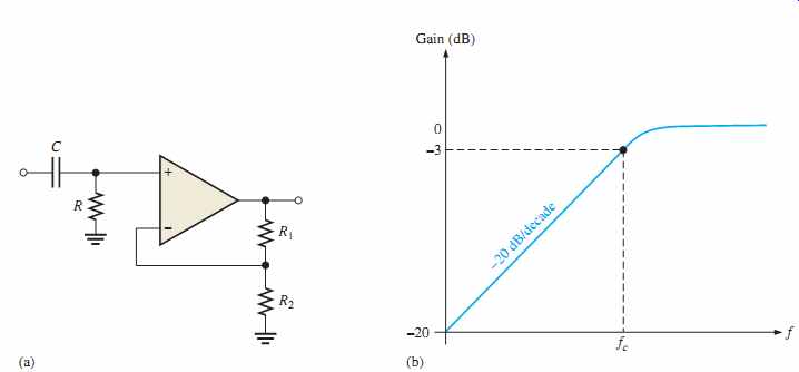

FIG. 13 Single-pole active high-pass filter and response curve.
Ideally, a high-pass filter passes all frequencies above fc without limit, as indicated in FIG. 14(a), although in practice, this is not the case. As you have learned, all op-amps inherently have internal RC circuits that limit the amplifier's response at high frequencies.
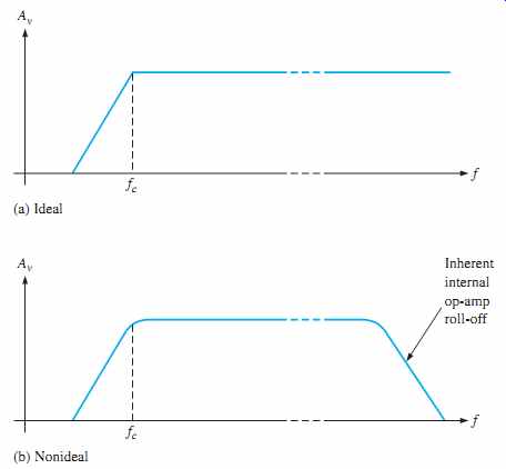
FIG. 14 High-pass filter response.
Therefore, there is an upper-frequency limit on the high-pass filter's response which, in effect, makes it a band-pass filter with a very wide bandwidth. In the majority of applications, the internal high-frequency limitation is so much greater than that of the filter's critical frequency that the limitation can be neglected. In some applications, discrete transistors are used for the gain element to increase the high-frequency limitation beyond that realizable with available op-amps.
The Sallen-Key High-Pass Filter
A high-pass Sallen-Key configuration is shown in FIG. 15. The components RA, CA, RB and CB, form the two-pole frequency-selective circuit. Notice that the positions of the resistors and capacitors in the frequency-selective circuit are opposite to those in the low-pass configuration. As with the other filters, the response characteristic can be optimized by proper selection of the feedback resistors, R1 and R2.
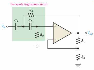
FIG. 15 Basic Sallen-Key high-pass filter.
Cascading High-Pass Filters
As with the low-pass configuration, first- and second-order high-pass filters can be cascaded to provide three or more poles and thereby create faster roll-off rates. FIG. 16 shows a six-pole high-pass filter consisting of three Sallen-Key two-pole stages. With this configuration optimized for a Butterworth response, a roll-off of -120 dB/decade is achieved.
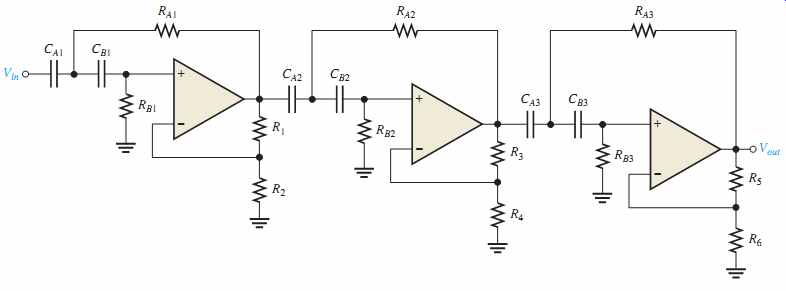
FIG. 16 Sixth-order high-pass filter.
SECTION 4 CHECKUP
1. How does a high-pass Sallen-Key filter differ from the low-pass configuration?
2. To increase the critical frequency of a high-pass filter, would you increase or decrease the resistor values?
3. If three two-pole high-pass filters and one single-pole high-pass filter are cascaded, what is the resulting roll-off?
5. ACTIVE BAND-PASS FILTERS
As mentioned, band-pass filters pass all frequencies bounded by a lower-frequency limit and an upper-frequency limit and reject all others lying outside this specified band. A band-pass response can be thought of as the overlapping of a low-frequency response curve and a high-frequency response curve.
After completing this section, you should be able to:
-- Analyze basic types of active band-pass filters
-- Describe how to cascade low-pass and high-pass filters to create a band-pass filter
-- Calculate the critical frequencies and the center frequency
-- Identify and analyze a multiple-feedback band-pass filter
-- Determine the center frequency, quality factor (Q), and bandwidth
-- Calculate the voltage gain
-- Identify and describe the state-variable filter
-- Explain the basic filter operation
-- Determine the Q
-- Identify and discuss the biquad filter
Cascaded Low-Pass and High-Pass Filters
One way to implement a band-pass filter is a cascaded arrangement of a high-pass filter and a low-pass filter, as shown in FIG. 17(a), as long as the critical frequencies are sufficiently separated. Each of the filters shown is a Sallen-Key Butterworth configuration so that the roll-off rates are -40 dB/decade, indicated in the composite response curve of FIG. 17(b). The critical frequency of each filter is chosen so that the response curves overlap sufficiently, as indicated. The critical frequency of the high-pass filter must be sufficiently lower than that of the low-pass stage. This filter is generally limited to wide band width applications.
The lower frequency fc1 of the passband is the critical frequency of the high-pass filter. The upper frequency fc2 is the critical frequency of the low-pass filter. Ideally, as discussed earlier, the center frequency f0 of the passband is the geometric mean of fc1 and fc2.
The following formulas express the three frequencies of the band-pass filter in FIG. 17.
Of course, if equal-value components are used in implementing each filter, the critical frequency equations simplify to the form fc = 1/(2 pi RC).
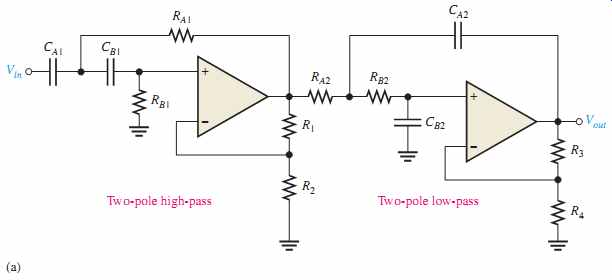
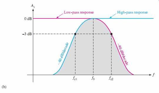

FIG. 17 Band-pass filter formed by cascading a two-pole high-pass and
a two-pole low-pass filter (it does not matter in which order the filters
are cascaded).
Multiple-Feedback Band-Pass Filter
Another type of filter configuration, shown in FIG. 18, is a multiple-feedback band pass filter. The two feedback paths are through R2 and C1. Components R1 and C1 provide the low-pass response, and R2 and C2 provide the high-pass response. The maximum gain, A0, occurs at the center frequency. Q values of less than 10 are typical in this type of filter.
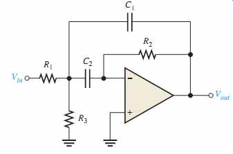
FIG. 18 Multiple-feedback band-pass filter.
An expression for the center frequency is developed as follows, recognizing that R1 and R3 appear in parallel as viewed from the C1 feedback path (with the Vin source replaced by a short).

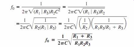
Equation 8
A value for the capacitors is chosen and then the three resistor values are calculated to achieve the desired values for f0, BW, and A0. As you know, the Q can be determined from the relation Q = f0/BWThe resistor values can be found using the following formulas (stated without derivation):
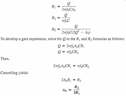
Equation 9
In order for the denominator of the equation R3 = Q/[2 pi f0 C (2Q^2 - A0)] to be positive, A0 < 2Q^2 which imposes a limitation on the gain.
State-Variable Filter
The state-variable or universal active filter is widely used for band-pass applications. As shown in FIG. 20, it consists of a summing amplifier and two op-amp integrators (which act as single-pole low-pass filters) that are combined in a cascaded arrangement to form a second-order filter. Although used primarily as a band-pass (BP) filter, the state variable configuration also provides low-pass (LP) and high-pass (HP) outputs. The center frequency is set by the RC circuits in both integrators. When used as a band-pass filter, the critical frequencies of the integrators are usually made equal, thus setting the center frequency of the passband.
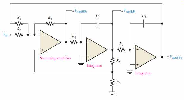
FIG. 20 State-variable filter.
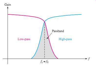
FIG. 21 General state-variable response curves.
Basic Operation
At input frequencies below fc, the input signal passes through the summing amplifier and integrators and is fed back 180° out of phase. Thus, the feedback signal and input signal cancel for all frequencies below approximately fc. As the low-pass response of the integrators rolls off, the feedback signal diminishes, thus allowing the input to pass through to the band-pass output. Above fc, the low-pass response disappears, thus preventing the input signal from passing through the integrators. As a result, the band-pass filter output peaks sharply at fc, as indicated in FIG. 21. Stable Qs up to 100 can be obtained with this type of filter. The Q is set by the feedback resistors R5 and R6 according to the following equation:

The state-variable filter cannot be optimized for low-pass, high-pass, and narrow band pass performance simultaneously for this reason: To optimize for a low-pass or a high-pass Butterworth response, DF must equal 1.414. Since Q = 1/DF, a Q of 0.707 will result.
Such a low Q provides a very wide band-pass response (large BW and poor selectivity). For optimization as a narrow band-pass filter, the Q must be set high.
The Biquad Filter
The biquad filter is similar to the state-variable filter except that it consists of an integrator, followed by an inverting amplifier, and then another integrator, as shown in FIG. 23. These differences in the configuration between a biquad and a state-variable filter result in some operational differences although both allow a very high Q value. In a biquad filter, the bandwidth is independent and the Q is dependent on the critical frequency; however, in the state-variable filter it is just the opposite: the bandwidth is dependent and the Q is independent on the critical frequency. Also, the biquad filter provides only band-pass and low-pass outputs.
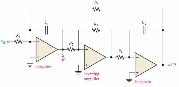
FIG. 23 A biquad filter.
SECTION 5 CHECKUP
1. What determines selectivity in a band-pass filter?
2. One filter has a Q = 5 and another has a Q = 25. Which has the narrower bandwidth?
3. List the active elements that make up a state-variable filter.
4. List the active elements that make up a biquad filter.