AMAZON multi-meters discounts AMAZON oscilloscope discounts
1. Corona Modes
In a nonuniform field gap in atmospheric air, corona discharges can develop over a whole range of volt ages in a small region near the highly stressed electrode before the gap breaks down. Several criteria have been developed for the onset of corona discharge, the most familiar being the streamer criterion.
They are all related to the development of an electron avalanche in the gas gap and can be expressed as …
Where …
α and η are, respectively, the ionization and attachment coefficients in air
α - η is the net coefficient of ionization by electron impact of the gas.
γ is a coefficient representing the efficiency of secondary processes in maintaining the ionization activities in the gap.
The net coefficient of ionization varies with the distance x from the highly stressed electrode and the integral is evaluated for values of x where a' is positive.
A physical meaning may be given to the corona onset criteria given earlier. The onset conditions can be rewritten as…
The left-hand side represents the avalanche development from a single electron and 1/γ the critical size of the avalanche to assure the stable development of the discharge.
The nonuniform field necessary for the development of corona discharges and the electronegative nature of air favor the formation of negative ions during the discharge development. Due to their relatively slow mobility, ions of both polarities from several consecutive electron avalanches accumulate in the low-field region of the gap and form ion space charges. To properly interpret the development of corona discharges, account must be taken of the active role of these ion space charges, which continuously modify the local field intensity and, hence, the development of corona discharges according to their relative buildup and removal from the region around the highly stressed electrode.

1.1 Negative Corona Modes
When the highly stressed electrode is at a negative potential, electron avalanches are initiated at the cathode and develop toward the anode in a continuously decreasing field. Referring to FIG. 1, the nonuniformity of the field distribution causes the electron avalanche to stop at the boundary surface S0, where the net ionization coefficient is zero, that is, a = ?. Since free electrons can move much faster than ions under the influence of the applied field, they concentrate at the avalanche head during its progression. A concentration of positive ions thus forms in the region of the gap between the cathode and the boundary surface, while free electrons continue to migrate across the gap. In air, free electrons rapidly attach themselves to oxygen molecules to form negative ions, which, because of the slow drift velocity, start to accumulate in the region of the gap beyond S0. Thus, as soon as the first electron avalanche has developed, there are two ion space charges in the gap.
The presence of these space charges increases the field near the cathode, but it reduces the field intensity at the anode end of the gap. The boundary surface of zero ionization activity is therefore displaced toward the cathode. The subsequent electron avalanche develops in a region of slightly higher field intensity but covers a shorter distance than its predecessor. The influence of the ion space charge is such that it actually conditions the development of the discharge at the highly stressed electrode, producing three modes of corona discharge with distinct electrical, physical, and visual characteristics ( FIG. 2). These are, respectively, with increasing field intensity: Trichel streamer, negative pulseless glow, and negative streamer. An interpretation of the physical mechanism of different corona modes is given in the following.
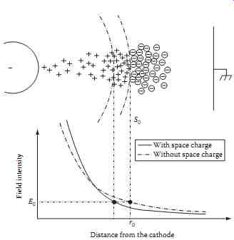
FIG. 1 Development of an electron avalanche from the cathode. (From
Trinh, N.G., IEEE Electr. Insul. Mag., 11, 23, 1995a.) Note: Distance
from the cathode
1.1.1 Trichel Streamer
FIG. 2 Corona modes at cathode: (a) Trichel streamers; (b) negative
pulseless glow; (c) negative streamers. Cathode: spherical protrusion
(d = 0.8 cm) on a sphere (D = 7 cm); gap 19 cm; time exposure 1/4 s.
(From Trinh, N.G. and Jordan, I.B., IEEE Trans., PAS-87, 1207, 1968;
From Trinh, N.G., IEEE Electr. Insul. Mag., 11, 23, 1995a.)
FIG. 2a shows the visual aspect of the discharge; its current and light characteristics are shown in FIG. 3. The discharge develops along a narrow channel from the cathode and follows a regular pattern in which the streamer is initiated, developed, and suppressed; a short dead time follows before the cycle is repeated. The duration of an individual streamer is very short, a few tens of nanoseconds, while the dead time varies from a few microseconds to a few milliseconds, or even longer. The resulting discharge current consists of regular negative pulses of small amplitude and short duration, succeeding one another at the rate of a few thousand pulses per second. A typical Trichel current pulse is shown in FIG. 3a where, it should be noted, the wave shape is somewhat influenced by the time constant of the measuring circuit.
The discharge duration may be significantly shorter, as depicted by the light pulse shown in FIG. 3c.
The development of Trichel streamers cannot be explained without taking account of the active roles of the ion space charges and the applied field. The streamer is initiated from the cathode by a free electron.
If the corona onset conditions are met, the secondary emissions are sufficient to trigger new electron avalanches from the cathode and maintain the discharge activity. During the streamer development, several generations of electron avalanches are initiated from the cathode and propagate along the streamer channel. The avalanche process also produces two ion space charges in the gap, which gradually moves the boundary surface S0 closer to the cathode. The positive ion cloud thus finds itself compressed at the cathode and, in addition, is partially neutralized at the cathode and by the negative ions produced in subsequent avalanches. This results in a net negative ion space charge, which eventually reduces the local field intensity at the cathode below the onset field and suppresses the discharge. The dead time is a period during which the remaining ion space charges are dispersed by the applied field. A new streamer will develop when the space charges in the immediate surrounding of the cathode have been cleared to a sufficient extent.
This mechanism depends on a very active electron attachment process to suppress the ionization activity within a few tens of nanoseconds following the beginning of the discharge. The streamer repetition rate is essentially a function of the removal rate of ion space charges by the applied field, and generally shows a linear dependence on the applied voltage. However, at high fields a reduction in the pulse repetition rate may be observed, which corresponds to the transition to a new corona mode.
1.1.2 Negative Pulseless Glow
The negative pulseless glow mode is characterized by a pulseless discharge current. As indicated by the well-defined visual aspect of the discharge ( FIG. 2b), the discharge itself is particularly stable, which shows the basic characteristics of a miniature glow discharge. Starting from the cathode, a cathode dark space can be distinguished, followed by a negative glow region, a Faraday dark space, and, finally, a positive column of conical shape. As with low-pressure glow discharges, these features of the pulseless glow discharge result from very stable conditions of electron emission from the cathode by ionic bombardment. The electrons, emitted with very low kinetic energy, are first propelled through the cathode dark space, where they acquire sufficient energy to ionize the gas, and intensive ionization occurs at the negative glow region. At the end of the negative glow region, the electrons lose most of their kinetic energy and are again accelerated across the Faraday dark space before they can ionize the gas atoms in the positive column. The conical shape of the positive column is attributed to the diffusion of the free electrons in the low-field region.
These stable discharge conditions may be explained by the greater efficiency of the applied field in removing the ion space charges at higher field intensities. Negative ion space charges cannot build up sufficiently close to the cathode to effectively reduce the cathode field and suppress the ionization activities there. This interpretation of the discharge mechanism is further supported by the existence of a plateau in the Trichel streamer current and light pulses ( FIG. 3), which indicates that an equilibrium state exists for a short time between the removal and the creation of the negative ion space charge. It has been shown (Trinh and Jordan, 1970) that the transition from the Trichel streamer mode to the negative pulseless glow corresponds to an indefinite prolongation in time of one such current plateau.
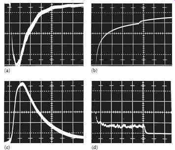
FIG. 3 Current and light characteristics of Trichel streamer. Cathode:
spherical protrusion (d = 0.8 cm) on a sphere (D = 7 cm); gap 19 cm.
Scales: (a) current 350 µA/div., 50 ns/div. (b) 50 µA/div., 2 µs/div.
Light: (c) 0.5 V/div., 20 ns/div. (d) 0.2 V/div., 2 µs/div. (From Trinh,
N.G. and Jordan, I.B., IEEE Trans., PAS-87, 1207, 1968; From Trinh, N.G.,
IEEE Electr. Insul. Mag., 11, 23, 1995a.)
1.1.3 Negative Streamer
If the applied voltage is increased still further, negative streamers may be observed, as illustrated in FIG. 2c. The discharge possesses essentially the same characteristics observed in the negative pulseless glow discharge but here the positive column of the glow discharge is constricted to form the streamer channel, which extends farther into the gap. The glow discharge characteristics observed at the cathode imply that this corona mode also depends largely on electron emissions from the cathode by ionic bombardment, while the formation of a streamer channel characterized by intensive ionization denotes an even more effective space charge removal action by the applied field. The streamer channel is fairly stable. It projects from the cathode into the gap and back again, giving rise to a pulsating fluctuation of relatively low frequency in the discharge current.
1.2 Positive Corona Modes
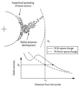 FIG.
4 Development of an electron avalanche toward the anode. (From Trinh,
N.G., IEEE Electr. Insul. Mag., 11, 23, 1995a.) Note: Distance from the
anode
FIG.
4 Development of an electron avalanche toward the anode. (From Trinh,
N.G., IEEE Electr. Insul. Mag., 11, 23, 1995a.) Note: Distance from the
anode
When the highly stressed electrode is of positive polarity, the electron avalanche is initiated at a point on the boundary surface S0 of zero net ionization and develops toward the anode in a continuously increasing field ( FIG. 4). As a result, the highest ionization activity is observed at the anode. Here again, due to the lower mobility of the ions, a positive ion space charge is left behind along the development path of the avalanche. However, because of the high field intensity at the anode, few electron attachments occur and the majority of free electrons created are neutralized at the anode. Negative ions are formed mainly in the low-field region farther in the gap. The following discharge behavior may be observed:
• The incoming free electrons are highly energetic and cannot be immediately absorbed by the anode. As a result, they tend to spread over the anode surface where they lose their energy through ionization of the gas particles, until they are neutralized at the anode, thus contributing to the development of the discharge over the anode surface.
• Since the positive ions are concentrated immediately next to the anode surface, they may produce a field enhancement in the gap that attracts secondary electron avalanches and promotes the radial propagation of the discharge into the gap along a streamer channel.
• During streamer discharge, the ionization activity is observed to extend considerably into the low field region of the gap via the formation of corona globules, which propagate owing to the action of the electric field generated by their own positive ion space charge. Dawson (1965) has shown that if a corona globule is produced containing 108 positive ions within a spherical volume of 3 × 10⁻³ cm in radius, the ion space charge field is such that it attracts sufficient new electron avalanches to create a new corona globule a short distance away. In the meantime, the initial corona globule is neutralized, causing the corona globule to effectively move ahead toward the cathode.
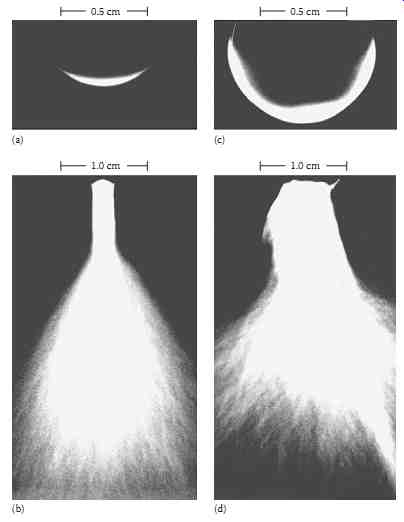
FIG. 5 Corona modes at anode: (a) burst corona; (b) onset streamers;
(c) positive glow corona; (d) break down streamers. Anode spherical protrusion
(d = 0.8 cm) on a sphere (D = 7 cm); gap 35 cm; time exposure 1/4 s. (From
Trinh, N.G. and Jordan, I.B., IEEE Trans., PAS-87, 1207, 1968; From Trinh,
N.G., IEEE Electr. Insul. Mag., 11, 23, 1995a.)
The presence of ion space charges of both polarities in the anode region greatly affects the local distribution of the field, and, consequently, the development of corona discharge at the anode. Four different corona discharge modes having distinct electrical, physical, and visual characteristics can be observed at a highly stressed anode, prior to flashover of the gap. These are, respectively, with increasing field intensity ( FIG. 5): burst corona, onset streamers, positive glow, and breakdown streamers. An interpretation of the physical mechanisms leading to the development of these corona modes is given in the following.
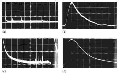
FIG. 6 (a) Burst corona current pulse. Scales: 5 mA/div., 0.2 ms/div.
(b) Development of burst corona following a streamer discharge. Scales:
5 mA/div., 0.2 ms/div. (c) Current characteristics of onset streamers.
Scales: 7 mA/div., 50 ns/div. (d) Light characteristics of onset streamers.
Scales: 1 V/div., 20 ns/div. (From Juette, G.W., IEEE Trans., PAS-91,
865, 1972; From Trinh, N.G. and Jordan, I.B., IEEE Trans., PAS-87, 1207,
1968; From Trinh, N.G., IEEE Electr. Insul. Mag., 11, 23, 1995a.)
1.2.1 Burst Corona
The burst corona appears as a thin luminous sheath adhering closely to the anode surface ( FIG. 5a). The discharge results from the spread of ionization activities at the anode surface, which allows the high-energy incoming electrons to lose their energy before neutralization at the anode. During this process, a number of positive ions are created in a small area over the anode, which builds up a local positive space charge and suppresses the discharge. The spread of free electrons then moves to another part of the anode. The resulting discharge current consists of very small positive pulses ( FIG. 6a), each corresponding to the ionization spreading over a small area at the anode and then being suppressed by the positive ion space charge produced.
1.2.2 Onset Streamer
The positive ion space charge formed adjacent to the anode surface causes a field enhancement in its immediate vicinity, which attracts subsequent electron avalanches and favors the radial development of onset streamers. This discharge mode is highly effective and the streamers are observed to extend farther into the low-field region of the gap along numerous filamentary channels, all originating from a common stem projecting from the anode ( FIG. 5b). During this development of the streamers, a considerable number of positive ions are formed in the low-field region. As a result of the cumulative effect of the successive electron avalanches and the absorption at the anode of the free electrons created in the discharge, a net residual positive ion space charge forms in front of the anode. The local gradient at the anode then drops below the critical value for ionization and suppresses the streamer discharge.
A dead time is consequently required for the applied field to remove the ion space charge and restore the proper conditions for the development of a new streamer. The discharge develops in a pulsating mode, producing a positive current pulse of short duration, high amplitude, and relatively low repetition rate due to the large number of ions created in a single streamer ( FIG. 6c and d).
It has been observed that these first two discharge modes develop in parallel over a small range of voltages following corona onset. As the voltage is increased, the applied field rapidly becomes more effective in removing the ion space charge in the immediate vicinity of the electrode surface, thus promoting the lateral spread of burst corona at the anode. In fact, burst corona can be triggered just a few microseconds after suppression of the streamer ( FIG. 6b). This behavior can be explained by the rapid clearing of the positive ion space charge at the anode region, while the incoming negative ions encounter a high-enough gradient to shed their electrons, thus providing the seeding free electrons to initiate new avalanches and sustain the ionization activity over the anode surface in the form of burst corona. The latter will continue to develop until it is again suppressed by its own positive space charge.
As the voltage is raised even higher, the burst corona is further enhanced by a more effective space charge removal action of the field at the anode. During the development of the burst corona, positive ions are created and rapidly pushed away from the anode. The accumulation of positive ions in front of the anode results in the formation of a stable positive ion space charge that prevents the radial development of the discharge into the gap. Consequently, the burst corona develops more readily, at the expense of the onset streamer, until the latter is completely suppressed. A new mode, the positive glow discharge, is then established at the anode.
1.2.3 Positive Glow
A photograph of a positive glow discharge developing at a spherical protrusion is presented in FIG. 5.
This discharge is due to the development of the ionization activity over the anode surface, which forms a thin luminous layer immediately adjacent to the anode surface, where intense ionization activity takes place. The discharge current consists of a direct current (DC) superimposed by a small pulsating component with a high repetition rate, in the hundreds of kilohertz range. By analyzing the light signals obtained with photomultipliers pointing to different regions of the anode, it may be found that the luminous sheath is composed of a stable central region, from there, bursts of ionization activity may develop and project the ionizing sheath outward and back again, continuously, giving rise to the pulsating current component.
The development of the positive glow discharge may be interpreted as resulting from a particular combination of removal and creation of positive ions in the gap. The field is high enough for the positive ion space charge to be rapidly removed from the anode, thus promoting surface ionization activity.
Meanwhile, the field intensity is not sufficient to allow radial development of the discharge and the formation of streamers. The main contribution of the negative ions is to supply the necessary triggering electrons to sustain ionization activity at the anode.
1.2.4 Breakdown Streamer
If the applied voltage is further increased, streamers are again observed and they eventually lead to breakdown of the gap. The development of breakdown streamers is preceded by local streamer spots of intense ionization activity, which may be seen moving slowly over the anode surface. The development of streamer spots is not accompanied by any marked change in the current or the light signal. Only when the applied field becomes sufficiently high to rapidly clear the positive ion space charges from the anode region does radial development of the discharge become possible, resulting in breakdown streamers.
Positive breakdown streamers develop more and more intensively with higher applied voltage and eventually cause the gap to break down. The discharge is essentially the same as the onset streamer type but can extend much farther into the gap. The streamer current is more intense and may occur at a higher repetition rate. A streamer crossing the gap does not necessarily result in gap breakdown, which proves that the filamentary region of the streamer is not fully conducting.
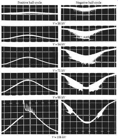
FIG. 7 Corona modes under AC voltage. Electrode: conical protrusion
(? = 30°) on a sphere (D = 7 cm); gap 25 cm; R = 10 k-ohm. Scales: 50
µA/div., 1.0 ms/div.
1.3 AC Corona
When alternating voltage is used, the gradient at the highly stressed electrode varies continuously, both in intensity and polarity. Different corona modes can be observed in the same cycle of the applied volt age. FIG. 7 illustrates the development of different corona modes at a spherical protrusion as a function of the applied voltage. The corona modes can be readily identified by the discharge current. The following observations can be made:
• For short gaps, the ion space charges created in one half-cycle are absorbed by the electrodes in the same half-cycle. The same corona modes that develop near onset voltages can be observed, namely, negative Trichel streamers, positive onset streamers, and burst corona.
• For long gaps, the ion space charges created in one half-cycle are not completely absorbed by the electrodes, leaving residual space charges in the gap. These residual space charges are drawn back to the region of high field intensity in the following half-cycle and can influence discharge development. Onset streamers are suppressed in favor of the positive glow discharge. The following corona modes can be distinguished: negative Trichel streamers, negative glow discharge, positive glow discharge, and positive breakdown streamers.
• Negative streamers are not observed under AC voltage, owing to the fact that their onset gradient is higher than the breakdown voltage that occurs during the positive half-cycle.
2 Main Effects of Corona Discharges on Overhead Lines
The impact of corona discharges on the design of HV lines has been recognized since the early days of electric power transmission when the corona losses (CLs) were the limiting factor. Even today, CLs remain critical for HV lines below 300 kV. With the development of EHV lines operating at voltages between 300 and 800 kV, RIs become the designing parameters. For UHV lines operating at voltages above 800 kV, the AN appears to gain in importance over the other two parameters. The physical mechanisms of these effects-CLs, RI, and AN-and their current evaluation methods are discussed later.
2.1 Corona Losses
The movement of ions of both polarities generated by corona discharges, and subjected to the applied field around the line conductors, is the main source of energy loss. For AC lines, the movement of the ion space charges is limited to the immediate vicinity of the line conductors, corresponding to their maxi mum displacement during one half-cycle, typically a few tens of centimeters, before the voltage changes polarity and reverses the ionic movement. For DC lines, the ion displacement covers the whole distance separating the line conductors, and between the conductors and the ground.
CLs are generally described in terms of the energy losses per kilometer of the line. They are generally negligible under fair-weather conditions but can reach values of several hundreds of kilowatts per kilo meter of line during foul weather. Direct measurement of CLs is relatively complex, but foul-weather losses can be readily evaluated in test cages under artificial rain conditions, which yield the highest energy loss. The results are expressed in terms of the generated loss W, a characteristic of the conductor to produce CLs under given operating conditions.
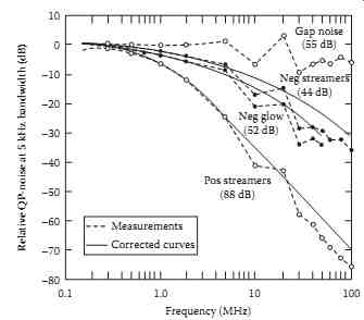
FIG. 8 Relative frequency spectra for different noise types.
2.2 Electromagnetic Interference
Electromagnetic interference is associated with streamer discharges that inject current pulses into the conductor. These pulses of steep front and short duration have a high harmonic content, reaching the tens of megahertz range, as illustrated in FIG. 8, which shows the typical frequency spectra associated with various streamer modes. A tremendous research effort was devoted to the subject during the years 1950-1980 in an effort to evaluate the RI from HV lines. The most comprehensive contributions were made by Moreau and Gary (1972a,b) of Électricité de France, who introduced the concept of the excitation function, G(?), which characterizes the ability of a line conductor to generate RI under the given operating conditions.
Consider first the case of a single-phase line, where the contribution to the RI at the measuring frequency, ?, from corona discharges developing at a section dx of the conductor is…
…where C is the capacitance per unit length of the line conductor to ground.
Upon injection, the discharge current pulse splits itself into two identical current pulses of half amplitude propagating in opposite directions away from the discharge site. At a point of observation located at a distance x along the line from the discharge site, the noise current is distorted according to…
…where ? represents the propagation constant, which can be approximated by its real component a.
The total noise current circulating in the line conductor is the sum of all contributions from the corona discharges along the conductor and is given by…
For a multiphase line, because of the high-frequency nature of the noise current, the calculation of the interference field must take account of the mutual coupling among the conductors, which further complicates the process (Gary, 1972; Moreau and Gary, 1972a,b). Modal analysis provides a convenient means of evaluating the noise currents on the line conductors. In this approach, the noise currents are first transposed into their modal components, which propagate without distortion along the line conductors at their own velocity according to the relation [M] is the modal transposition matrix j0(?) are the modal components of the injected noise current
The modal current at the measuring point located at a distance x from the injection point is
and the modal current component at the measuring point is…
2.2.1 Television Interference
The frequency spectrum of corona discharges has cut-off frequencies around a few tens of megahertz.
As a result, the interference levels at the television frequencies are very much attenuated. In fact, gap discharges, which generate sharp current pulse with nanosecond rise times, are the principal discharges that effectively interfere with the television reception. These discharges are produced by loose connections, a problem common on low-voltage distribution lines but rarely observed on HV transmission lines. Another source of interference is related to reflections of television signals at HV line towers, producing ghost images. However, the problem is not related in any way to corona activities on the line conductors.
2.3 Audible Noise
The high temperature in the discharge channel produced by the streamer creates a corresponding increase in the local air pressure. Consequently, a pulsating sound wave is generated from the discharge site, propagates through the surrounding ambient air, and is perfectly audible in the immediate vicinity of the HV lines. The typical octave-band frequency spectra of line corona in FIG. 9 contain discrete components corresponding to the second and higher harmonics of the line voltage superimposed on a relatively broadband noise, extending well into the ultrasonic range. The octave-band measurements in this figure show a sharp drop at frequencies over 20 kHz, due principally to the limited frequency response of the microphone and associated sound-level meter.
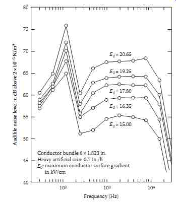 FIG. 9 Octave-band frequency spectra of line corona audible noise at
10 m from the conductor.
FIG. 9 Octave-band frequency spectra of line corona audible noise at
10 m from the conductor.
Similar to the case of RI, the ability of the line conductors to produce AN is characterized by the generated acoustic power density A, defined as the acoustic power produced per unit length of the line conductor under specific operating conditions. The acoustic power generated by corona discharges developing in a portion dx of the conductor is then
Its contribution to the acoustic intensity at a measuring point located at a distance r from the discharge site is…
The acoustic intensity at the measuring point is the sum of all contributions from corona discharge distributed along the conductor:
R is the distance from the measuring point to the conductor the integral is evaluated in terms of the longitudinal distance x along the conductor.
Finally, the acoustic intensity at the measuring point is the sum of the contributions from the different phase conductors of the line.
The sound pressure, usually expressed in terms of decibel (dBA) above a reference level of 2 × 10^-5.
2.4 Example of Calculation
It is obvious from the preceding sections that the effects of corona discharges on HV lines-the CLs, the RIs, and AN-can be readily evaluated from the generated loss W, the excitation function G(?), and the generated acoustic power density A of the conductor. The latter parameters are characteristics of the bundle conductor and are usually derived from tests in a test cage or on experimental line. An example calculation of the corona performance of an HV line is given in the following for the case of the Hydro-Québec's 735 kV lines under conditions of heavy rain. The line parameters are given in Table 1, together with the various corona-generated parameters taken from Trinh and Maruvada (1977). The calculation of the radio interference and AN levels will be made for a lateral distance of 15 m from the outer phase, i.e., at the limit of the right-of-way of the line.
Corona losses: The CLs are the sum of the losses generated at the three phases of the line, which amount to 127.63 kW/km.
TABLE 1 Hydro-Québec 735 kV Line
The corresponding electric interference level is 25.911 dB above 1 µV/m.
The aforementioned electric interference field and interference level are obtained assuming a noise excitation function of 1 0 . µ?/ m. For the case of interest, the excitation function at phase A is 39.59 dB and the corresponding interference level is 64.98 dB. By repeating the same process for the noise cur rents injected in phases B and C, one obtains effectively three sets of magnetic and electric field components generated by the circulation of the noise currents on the line conductors:
Their contributions to the noise level are, respectively, 64.26 and 64.98 dB, resulting in a total noise level of 69.53 dB at the measuring point. The measuring frequency is 0.5 MHz.
Audible noise: Calculation of the AN is straightforward, since each phase of the line can be considered as an independent noise source. Consider the AN generated from phase A. The sub-conductor-generated acoustic power density is -0.24 dBA or 1.58 × 10^-5 µW/m for the bundle conductor. The acoustic intensity at 15 m from the outer phase of the line as given by Equation 16.18 is 3.19 × 10^-7 W/m^2 and the noise level is 55.14 dBA above 2 × 10^-5 N/m^2.
By repeating the process for the other two phases of the line, the contributions to the acoustic intensity at the measuring point from the phases B and C of the line are 2.64 × 10^-7 and 1.69 × 10⁻⁷ W/m^2 , respectively, and the corresponding noise levels are 54.33 and 52.38 dBA. The total noise level is 58.87 dBA.
3 Impact on the Selection of Line Conductors
3.1 Corona Performance of HV Lines
Corona performance is a general term used to characterize the three main effects of corona discharges developing on the line conductors and their related hardware, namely, CLs, RI, and AN. All are sensitive to weather conditions, which dictate the corona activities. CLs can be described by a lump figure, which is equal to the total energy losses per kilometer of the line. Both the RI and the AN levels vary with the distance from the line and are best described by lateral profiles, which show the variations in the RI and AN level with the lateral distance from the line. Typical lateral profiles are presented in Figures 10 and 11 for a number of HV lines under foul-weather conditions. For convenience, the interference and noise levels at the edge of the right-of-way, typically 15 m from the outside phases of the line, are generally used to quantify the interference and noise level.
The time variations in the corona performance of HV lines is best described in terms of a statistical distribution, which shows the proportion of time that the energy losses, the RI, and AN exceed their specified levels. FIG. 12 illustrates typical corona performances of Hydro-Québec's 735 kV lines as measured at the edge of the right-of-way. It can be seen that the RI and AN levels vary over wide ranges. In addition, the cumulative distribution curves show a typical inverted-S shape, indicating that the recorded data actually result from the combination of more than one population, usually associated with fair- and foul-weather conditions.
DC coronas are less noisy than AC coronas. In effect, although DC lines can become very lossy during foul weather, the radio interference and ANs are significantly reduced. This behavior is related to the fact that water drops become elongated, remain stable, and produce glow corona modes rather than streamers in a DC field.
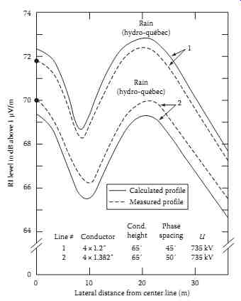
FIG. 10 Comparison of calculated and measured RI performances of Hydro-Québec
735 kV lines at 1 MHz and using natural modes.
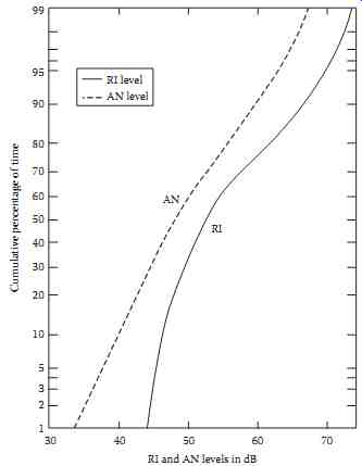
FIG. 11 Comparison of calculated and measured AN performances of HV
lines.
3.2 Approach to Control the Corona Performance
The occurrence of corona discharges on line conductors is dictated essentially by the local field intensity, which, in turn, is greatly affected by the surface conditions, e.g., rugosity, water drops, snow, and ice particles, etc. For a smooth cylindrical conductor, the corona onset field is well described by Peek's experimental law...
Ec is the corona onset field
a is the radius of the conductor
m is an experimental factor to take account of the surface conditions
Typical values of m are 0.8-0.9 for a dry-aged conductor, 0.5-0.7 for a conductor under foul-weather conditions, and d is the relative air density factor.
The aforementioned corona onset condition emphasizes the great sensitivity of corona activities to the conductor surface condition and, hence, to changes in weather conditions. In effect, although the line voltage and the nominal conductor surface gradient remain constant, the surface condition factor varies continuously due to the exposure of line conductors to atmospheric conditions. The changes are particularly pronounced during foul weather as a result of the numerous discharge sites associated with water drops, snow, and ice particles deposited on the conductor surface.
Adequate corona performance of HV lines is generally achieved by a proper control of the field intensity at the surface of the conductor. It can be well illustrated by the simple case of a single-phase, single conductor line for which the field intensity at the conductor surface is
It can be seen that the field intensity at the conductor surface is inversely proportional to its radius and, to a lesser extent, to the height of the conductor aboveground. By properly dimensioning the conductor, the field intensity at its surface can be kept below the fair-weather corona onset field for an adequate control of the corona activities and their undesirable effects.
FIG. 12 Cumulative distribution of RI and AN levels measured at 15
m from the outer phases of Hydro Québec 735 kV lines. (From Trinh, N.G.,
IEEE Electr. Insul. Mag., 11, 5, 1995b.)
With the single-conductor configuration, the size required for the conductor to be corona-free under fair-weather conditions is roughly proportional to the line voltage, and consequently will reach unrealistic values when the latter exceeds some 400 kV. Introduced in 1910 by Whitehead to increase the transmission capability of overhead lines (Whitehead, 1910), the concept of bundled conductors quickly revealed itself as an effective means of controlling the field intensity at the conductor surface, and hence, the line corona activities. This is well illustrated by the results in Table 16.2, which compare the single conductor design required to match the bundle performances in terms of power transmission capabilities, and the maximum conductor surface gradient for different line voltages. Bundled conductors are now used extensively in EHV lines rated 315 kV and higher; as a matter of fact, HV lines as we know them today would not exist without the introduction of conductor bundles.
3.3 Selection of Line Conductors
Even with the use of bundled conductors, it is not economically justifiable to design line conductors that would be corona-free under all weather conditions. The selection of line conductors is therefore made in terms of them being relatively corona-free under fair weather. While corona activities are tolerated under foul weather, their effects are controlled to acceptable levels at the edge of the right-of-way of the line. For AC lines, the design levels of 70 dB for the radio interference and 60 dBA for the AN at the edge of the right-of-way are often used (Trinh et al., 1974). These levels may be reached during periods of foul weather, and for a specified annual proportion of time, typically 15%-20%, depending on the local distribution of the weather pattern. The design process involves extensive field calculations and experimental testing to determine the number and size of the line conductors required to minimize the undesirable effects of corona discharges. Current practices in dimensioning HV-line conductors usually involve two stages of selection according to their worst-case and long-term corona performances.
TABLE 2 Comparison of Single and Bundled Conductors' Performances
Line voltage (kV) 400 735 1100
Distance between phases (m) 12 13.7 17
Number of sub-conductors 2 4 8
Bundle diameter (cm) 45 65 84
Conductor diameter (cm) 3.2 3.05 3.2
Corona onset gradient, m = 0.85, (kVrms/cm) 22.32 22.04 22.32
Maximum surface gradient (kVrms/cm) 16.3 19.79 17.3
Single conductor diameter of the same gradient (cm) 4.7 8.5 13.8
Transmission capability (GW) 0.5 2.0 4.9
Single conductor diameter of the same transmission capability (cm) 8.5 22 64
3.3.1 Worst-Case Performance
Several conductor configurations (number, spacing, and diameter of the sub-conductors) are selected with respect to their worst-case performances which, for AC lines, correspond to foul-weather conditions, in particular heavy rain. Evaluation of the conductor worst-case performance is best done in test cages under artificial heavy rain conditions. Test cages of square section, typically 3 m × 3 m, and a few tens of meters long, are adequate for evaluating full-size conductor bundles located along its central axis, for lines up to the 1500 kV class. The advantages of this experimental setup are the relatively modest test voltage required to reproduce the same field distribution on real-size bundled conductors, and the possibility of artificially producing the heavy rain conditions. The worst case performance of various bundled conductors as defined by their generating quantities, namely, the corona-generated losses W, the RI excitation function G, and the AN-generated acoustic power density A, can then be determined over a wide range of surface gradients.
Under DC voltage, the worst-case corona performance is not directly related to foul-weather conditions. Although heavy rain was found to produce the highest losses, both the RI and the AN levels decrease under rain conditions. This behavior is related to the fact that under DC field conditions, the water droplets have an optimum shape, favorable to the development of stable glow-corona modes. For this reason, test cage is less effective in evaluating the worst-case DC performance of bundled conductors.
A significant amount of data were gathered in cage tests at IREQ during the 1970s and provided the database for the development of a method to predict the worst-case performance of bundled conductors for AC voltage. The latter was based on the following considerations:
• The corona performances of single conductors under artificial heavy rain conditions, as expressed by the generating functions, are a function of the conductor diameter and of the field intensity at its surface and can be expressed by the following empirical formula:
Gs(dB) = -93.35 + 92.42 log(E) + 43.03 log(d) for the excitation function, Gs,
As(dB) = -123.94 + 82.84 log(E) + 48.28 log(d) for the generated acoustic power density, As, and for the corona-generated losses Ws.
…where E is expressed in kVrms/cm and d is in cm.
The field intensity at the surface of a sub-conductor in a bundle is a function of its position and can be expressed as…
alpha is the angle defining a point at the sub-conductor surface with respect to the point of maxi mum field intensity;
f is the angle defining a point at the sub-conductor surface with respect to the horizontal axis a is the angle of the point of maximum field intensity at the sub-conductor surface, with respect to the horizontal axis;
Ea is the average field intensity;
delta E is the difference between the extreme field intensities at the subconductor surface Noting that for a given bundle conductor, the subconductor diameter is known, and the corona performances of the single conductor become a function of the field intensity at its surface only. As a result, the corona generating quantities of a bundle conductor under the actual operating conditions can be derived from that of the single conductor of the same size as the subconductor of the bundle, and taking into account of the actual distribution of the field intensity at the surface of the subconductors. The following expressions are obtained for the various generating quantities:
For the RI excitation function, Gb:
where Cs and Cb are, respectively, the capacitances of the single conductor and the bundle conductor in the test cage.
Once the generating quantities are determined, the worst-case corona performances of the line can be evaluated as described in previous sections. The results presented in Figures 16.10 and 16.11, which compare the calculated and measured lateral RI and AN profiles of a number of HV lines, illustrate the good concordance of this approach. Commercial software exist that evaluate the worst-case performance of HV-line conductors using available experimental data obtained in cage tests under conditions of artificial heavy rain, making it possible to avoid undergoing tedious and expensive tests to help select the best configurations for line conductors for a given rating of the line.
3.3.2 Long-Term Corona Performance
Because of their wide range of variation in different weather conditions, representative corona performances of HV line are best evaluated in their natural environment. Test lines are generally used in this study that involves energizing the conductors for a sufficiently long period, usually 1 year to cover most of the weather conditions, and recording their corona performances together with the weather conditions. The higher cost of the long-term corona performance study usually limits its application to a small number of conductor configurations selected from their worst-case performance.
It should be noted that best results for the long-term corona performance evaluated on test lines are obtained when the weather pattern at the test site is similar to that existing along the actual HV line. A direct transposition of the results is then possible. If this condition is not met, some interpretation of the experimental data is needed. This is done by first decomposing the recorded long-term data into two groups, corresponding to the fair- and foul-weather conditions, then recombining these data according to the local weather pattern to predict the long-term corona performance along the line.
4 Conclusions
This section on transmission systems has reviewed the physics of corona discharges and discussed their impact on the design of HV lines, specifically in the selection of the line conductors. The following conclusions can be drawn.
Corona discharges can develop in different modes, depending on the equilibrium state existing under a given test condition, between the buildup and removal of ion space charges from the immediate vicinity of the highly stressed electrode. Three different corona modes-Trichel streamer, negative glow, and negative streamer-can be observed at the cathode with increasing applied field intensities. With positive polarity, four different corona modes are observed, namely, burst corona, onset streamers, positive glow, and breakdown streamers.
While all corona modes produce energy losses, the streamer discharges also generate RI and AN in the immediate vicinity of HV lines. These parameters are currently used to evaluate the corona performance of conductor bundles and to predict the energy losses and environmental impact of HV lines before their installation.
Adequate control of line corona is obtained by controlling the surface gradient at the line conductors.
The introduction of bundled conductors in 1910 has greatly influenced the development of HV lines to today's EHVs.
Also see...
ElectricalNotes article: What is the corona efect