AMAZON multi-meters discounts AMAZON oscilloscope discounts
The energized conductors of transmission and distribution lines must be placed to totally eliminate the possibility of injury to people. Overhead conductors, however, elongate with time, temperature, and tension, thereby changing their original positions after installation. Despite the effects of weather and loading on a line, the conductors must remain at safe distances from buildings, objects, and people or vehicles passing beneath the line at all times. To ensure this safety, the shape of the terrain along the right-of-way, the height and lateral position of the conductor support points, and the position of the conductor between support points under all wind, ice, and temperature conditions must be known.
Bare overhead transmission or distribution conductors are typically quite flexible and uniform in weight along their length. Because of these characteristics, they take the form of a catenary between support points. The shape of the catenary changes with conductor temperature, ice and wind loading, and time. To ensure adequate vertical and horizontal clearance under all weather and electrical loadings, and to ensure that the breaking strength of the conductor is not exceeded, the behavior of the conductor catenary under all conditions must be known before the line is designed. The future behavior of the conductor is determined through calculations commonly referred to as sag-tension calculations.
Sag-tension calculations predict the behavior of conductors based on recommended tension limits under varying loading conditions. These tension limits specify certain percentages of the conductor's rated breaking strength that are not to be exceeded upon installation or during the life of the line. These conditions, along with the elastic and permanent elongation properties of the conductor, provide the basis for determining the amount of resulting sag during installation and long-term operation of the line.
Accurately determined initial sag limits are essential in the line design process. Final sags and tensions depend on initial installed sags and tensions and on proper handling during installation. The final sag shape of conductors is used to select support point heights and span lengths so that the mini mum clearances will be maintained over the life of the line. If the conductor is damaged or the initial sags are incorrect, the line clearances may be violated or the conductor may break during heavy ice or wind loadings.
1. Catenary Cables
A bare-stranded overhead conductor is normally held clear of objects, people, and other conductors by periodic attachment to insulators. The elevation differences between the supporting structures affect the shape of the conductor catenary. The catenary's shape has a distinct effect on the sag and tension of the conductor, and therefore, must be determined using well-defined mathematical equations.
1.1 Level Spans
The shape of a catenary is a function of the conductor weight per unit length, w, the horizontal component of tension, H, span length, S, and the maximum sag of the conductor, D. Conductor sag and span length are illustrated in FIG. 1 for a level span.
The exact catenary equation uses hyperbolic functions. Relative to the low point of the catenary curve shown in FIG. 1, the height of the conductor, y(x), above this low point is given by the following equation:
Note that x is positive in either direction from the low point of the catenary. The expression to the right is an approximate parabolic equation based upon a MacLaurin expansion of the hyperbolic cosine.
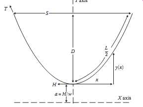
Above: Fig. 1 Catenary curve for level spans.
For a level span, the low point is in the center, and the sag, D, is found by substituting x = S/2 in the preceding equations. The exact and approximate parabolic equations for sag become the following:
The ratio, H/w, which appears in all of the preceding equations, is commonly referred to as the catenary constant. An increase in the catenary constant, having the units of length, causes the catenary curve to become shallower and the sag to decrease. Although it varies with conductor temperature, ice, and wind loading, and time, the catenary constant typically has a value in the range of several thousand feet for most transmission-line catenaries.
The approximate or parabolic expression is sufficiently accurate as long as the sag is <5% of the span length. As an example, consider a 1000 ft span of Drake conductor (w = 1.096 lb/ft) installed at a tension of 4500 lb. The catenary constant equals 4106 ft. The calculated sag is 30.48 and 30.44 ft using the hyperbolic and approximate equations, respectively. Both estimates indicate a sag-to-span ratio of 3.4% and a sag difference of only 0.5 in.
The horizontal component of tension, H, is equal to the conductor tension at the point in the catenary where the conductor slope is horizontal. For a level span, this is the midpoint of the span length. At the ends of the level span, the conductor tension, T, is equal to the horizontal component plus the conductor weight per unit length, w, multiplied by the sag, D, as shown in the following:
Given the conditions in the preceding example calculation for a 1000 ft level span of Drake ACSR, the tension at the attachment points exceeds the horizontal component of tension by 33 lb. It’s common to perform sag-tension calculations using the horizontal tension component, but the average of the horizontal and support point tension is usually listed in the output.
1.2 Conductor Length
Application of calculus to the catenary equation allows the calculation of the conductor length, L(x), measured along the conductor from the low point of the catenary in either direction.
The resulting equation becomes
For a level span, the conductor length corresponding to x = S/2 is half of the total conductor length and the total length, L, is...
The parabolic equation for conductor length can also be expressed as a function of sag, D, by substitution of the sag parabolic equation, giving
1.3 Conductor Slack
The difference between the conductor length, L, and the span length, S, is called slack. The parabolic equations for slack may be found by combining the preceding parabolic equations for conductor length, L, and sag, D:
While slack has units of length, it’s often expressed as the percentage of slack relative to the span length.
Note that slack is related to the cube of span length for a given H/w ratio and to the square of sag for a given span. For a series of spans having the same H/w ratio, the total slack is largely determined by the longest spans. It’s for this reason that the ruling span (RS) is nearly equal to the longest span rather than the average span in a series of suspension spans.
Equation 7 can be inverted to obtain a more interesting relationship showing the dependence of sag, D, upon slack, L - S:
As can be seen from the preceding equation, small changes in slack typically yield large changes in conductor sag.
1.4 Inclined Spans
Inclined spans may be analyzed using essentially the same equations that were used for level spans. The catenary equation for the conductor height above the low point in the span is the same. However, the span is considered to consist of two separate sections, one to the right of the low point and the other to the left as shown in FIG. 2. The shape of the catenary relative to the low point is unaffected by the difference in suspension point elevation (span inclination).
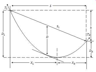
Above: Fig. 2 Inclined catenary span.
In each direction from the low point, the conductor elevation, y(x), relative to the low point is given by...
...Note that x is considered positive in either direction from the low point.
The horizontal distance, xL, from the left support point to the low point in the catenary is ...
The horizontal distance, xR, from the right support point to the low point of the catenary is....
....where S is the horizontal distance between support points h is the vertical distance between support points D is the sag measured vertically from a line through the points of conductor support to a line tangent to the conductor The midpoint sag, D, is approximately equal to the sag in a horizontal span equal in length to the inclined span, Sl.
Knowing the horizontal distance from the low point to the support point in each direction, the pre ceding equations for y(x), L, D, and T can be applied to each side of the inclined span.
The total conductor length, L, in the inclined span is equal to the sum of the lengths in the xR and xL sub-span sections:
In each sub-span, the sag is relative to the corresponding support point elevation:
....or in terms of sag, D, and the vertical distance between support points:
...and the maximum tension is....
...or in terms of upper and lower support points:
where…
DR is the sag in right sub-span section DL is the sag in left sub-span section TR is the tension in right sub-span section TL is the tension in left sub-span section Tu is the tension in conductor at upper support Tl … is the tension in conductor at lower support
The horizontal conductor tension is equal at both supports. The vertical component of conductor tension is greater at the upper support and the resultant tension, Tu, is also greater.
1.5 Ice and Wind Conductor Loads
When a conductor is covered with ice and/or is exposed to wind, the effective conductor weight per unit length increases. During occasions of heavy ice and/or wind load, the conductor catenary tension increases dramatically along with the loads on angle and dead-end structures. Both the conductor and its supports can fail unless these high-tension conditions are considered in the line design.
The National Electric Safety Code (NESC) suggests certain combinations of ice and wind corresponding to heavy, medium, and light loading regions of the United States. FIG. 3 is a map of the United States indicating those areas (NESC, 2007). The combinations of ice and wind corresponding to loading region are listed in TBL. 1.
The NESC also suggests that increased conductor loads due to high wind loads without ice be considered. FIG. 4 shows the suggested wind pressure as a function of geographical area for the United States (ASCE Std. 7-88).
Certain utilities in very heavy ice areas use glaze ice thicknesses of as much as 2 in. to calculate iced conductor weight. Similarly, utilities in regions where hurricane winds occur may use wind loads as high as 34 lb/ft2
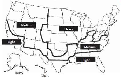
Above: Fig. 3 Ice and wind load areas of the United States.
TBL. 1 Definitions of Ice and Wind Load for NESC Loading Areas
As the NESC indicates, the degree of ice and wind loads varies with the region. Some areas may have heavy icing, whereas some areas may have extremely high winds. The loads must be accounted for in the line design process so they don’t have a detrimental effect on the line. Some of the effects of both the individual and combined components of ice and wind loads are discussed in the following.
1.5.1 Ice Loading
The formation of ice on overhead conductors may take several physical forms (glaze ice, rime ice, or wet snow). The impact of lower density ice formation is usually considered in the design of line sections at high altitudes.
The formation of ice on overhead conductors has the following influence on line design:
• Ice loads determine the maximum vertical conductor loads that structures and foundations must withstand.
• In combination with simultaneous wind loads, ice loads also determine the maximum transverse loads on structures.
• In regions of heavy ice loads, the maximum sags and the permanent increase in sag with time (difference between initial and final sags) may be due to ice loadings.
Ice loads for use in designing lines are normally derived on the basis of past experience, code requirements, state regulations, and analysis of historical weather data. Mean recurrence intervals for heavy ice loadings are a function of local conditions along various routings. The impact of varying assumptions concerning ice loading can be investigated with line design software.
The calculation of ice loads on conductors is normally done with an assumed glaze ice density of 57 lb/ft^3.
The weight of ice per unit length is calculated with the following equation:
....where t is the thickness of ice, in.
D_c is the conductor outside diameter, in.
W_ice is the resultant weight of ice, lb/ft
Above: Fig. 4 Wind pressure design values in the United States. Maximum recorded wind speed in miles/hour. (From Overend, P.R. and Smith, S., Impulse Time Method of Sag Measurement, American Society of Civil Engineers, Reston, VA, 1986.)
TBL. 2 Ratio of Iced to Bare Conductor Weight
The ratio of iced weight to bare weight depends strongly upon conductor diameter. As shown in TBL. 2 for three different conductors covered with 0.5 in. radial glaze ice, this ratio ranges from 4.8 for #1/0 AWG to 1.6 for 1590 kcmil conductors. As a result, small diameter conductors may need to have a higher elastic modulus and higher tensile strength than large conductors in heavy ice and wind loading areas to limit sag ( FIG. 5).
1.5.2 Wind Loading
Wind loadings on overhead conductors influence line design in a number of ways:
• The maximum span between structures may be determined by the need for horizontal clearance to edge of right-of-way during moderate winds.
• The maximum transverse loads for tangent and small angle suspension structures are often determined by infrequent high wind-speed loadings.
• Permanent increases in conductor sag may be determined by wind loading in areas of light ice load.
Wind pressure load on conductors, Pw, is commonly specified in lb/ft^2
. The relationship between Pw and wind velocity is given by the following equation:
… where V_w is the wind speed in miles per hour.
The wind load per unit length of conductor is equal to the wind pressure load, Pw, multiplied by the conductor diameter (including radial ice of thickness t, if any), is given by the following equation:
Above: Fig. 5 Sag-tension solution for 600 ft span of Drake at 0°F and 0.5 in. ice.
1.5.3 Combined Ice and Wind Loading
If the conductor weight is to include both ice and wind loading, the resultant magnitude of the loads must be determined vectorially. The weight of a conductor under both ice and wind loading is given by the following equation:
....where
wb is the bare conductor weight per unit length, lb/ft
wi is the weight of ice per unit length, lb/ft
ww is the wind load per unit length, lb/ft
ww+I is the resultant of ice and wind loads, lb/ft
The NESC prescribes a safety factor, K, in lb/ft, dependent upon loading district, to be added to the resultant ice and wind loading when performing sag and tension calculations. Therefore, the total resultant conductor weight, w, is…
1.6 Conductor Tension Limits
The NESC recommends limits on the tension of bare overhead conductors as a percentage of the conductor's rated breaking strength. The tension limits are 60% under maximum ice and wind load, 33.3% initial unloaded (when installed) at 60°F, and 25% final unloaded (after maximum loading has occurred) at 60°F. It’s common, however, for lower unloaded tension limits to be used. Except in areas experiencing severe ice loading, it’s not unusual to find tension limits of 60% maximum, 25% unloaded initial, and 15% unloaded final. This set of specifications could easily result in an actual maximum tension on the order of only 35%-40%, an initial tension of 20% and a final unloaded tension level of 15%. In this case, the 15% tension limit is said to govern.
Transmission-line conductors are normally not covered with ice, and winds on the conductor are usually much lower than those used in maximum load calculations. Under such everyday conditions, tension limits are specified to limit aeolian vibration to safe levels. Even with everyday lower tension levels of 15%-20%, it’s assumed that vibration control devices will be used in those sections of the line that are subject to severe vibration. Aeolian vibration levels, and thus appropriate unloaded tension limits, vary with the type of conductor, the terrain, span length, and the use of dampers. Special conductors, such as ACSS, SDC, and VR, exhibit high self-damping properties and may be installed to the full code limits, if desired.
2 Approximate Sag-Tension Calculations
Sag-tension calculations, using exacting equations, are usually performed with the aid of a computer; however, with certain simplifications, these calculations can be made with a handheld calculator. The latter approach allows greater insight into the calculation of sags and tensions than is possible with complex computer programs. Equations suitable for such calculations, as presented in the preceding section, can be applied to the following example:
It’s desired to calculate the sag and slack for a 600 ft level span of 795 kcmil-26/7 ACSR "Drake" conductor. The bare conductor weight per unit length, wb, is 1.094 lb/ft. The conductor is installed with a horizontal tension component, H, of 6,300 lb, equal to 20% of its rated breaking strength of 31,500 lb.
By the use of Equation 15.2, the sag for this level span is ...
The length of the conductor between the support points is determined using Equation 15.6:....
Note that the conductor length depends solely on span and sag. It’s not directly dependent on conductor tension, weight, or temperature. The conductor slack is the conductor length minus the span length; in this example, it’s 0.27 ft (0.0826 m).
2.1 Sag Change with Thermal Elongation
ACSR and AAC conductors elongate with increasing conductor temperature (TBL. 3). The rate of linear thermal expansion for the composite ACSR conductor is less than that of the AAC conductor because the steel strands in the ACSR elongate at approximately half the rate of aluminum. The effective linear thermal expansion coefficient of a non-homogenous conductor, such as Drake ACSR, may be found from the following equations:
Where…
EAL is the Elastic modulus of aluminum, psi EST is the Elastic modulus of steel, psi EAS is the Elastic modulus of aluminum-steel composite, psi AAL is the Area of aluminum strands, square units AST is the Area of steel strands, square units ATOTAL is the Total cross-sectional area, square units aAL is the Aluminum coefficient of linear thermal expansion, per °F aST is the Steel coefficient of thermal elongation, per °F aAS is the Composite aluminum-steel coefficient of thermal elongation, per °F
TBL. 3 Iterative Solution for Increased Conductor Temperature
The elastic modulus for solid aluminum wire is 10 million psi and for steel wire is 30 million psi. The elas tic modulus for stranded wire is reduced. The modulus for stranded aluminum is assumed to be 8.6 million psi for all strandings. The modulus for the steel core of ACSR conductors varies with stranding as follows:
• 27.5 × 10^6
for single-strand core
• 27.0 × 10^6
for 7-strand core
• 26.5 × 10^6
for 19-strand core
Using elastic moduli of 8.6 and 27.0 million psi for aluminum and steel, respectively, the elastic modulus for Drake ACSR is ...
....
If the conductor were inextensible, that is, if it had an infinite modulus of elasticity, then these values of sag and tension for a conductor temperature of 167°F would be correct. For any real conductor, however, the elastic modulus of the conductor is finite and changes in tension do change the conductor length.
The use of the preceding calculation, therefore, will overstate the increase in sag (FIG. 6).
The preceding approximate tension calculations could have been more accurate with the use of actual stress-strain curves and graphic sag-tension solutions, as described in detail in Graphic Method for Sag
Above: Fig. 6 Sag-tension solution for 600 ft span of Drake at 167°F.
Tension Calculations for ACSR and Other Conductors (Aluminum Company of America, 1961). This method, although accurate, is very slow and has been replaced completely by computational methods.
3. Numerical Sag-Tension Calculations
Sag-tension calculations are normally done numerically and allow the user to enter many different loading and conductor temperature conditions. Both initial and final conditions are calculated and multiple tension constraints can be specified. The complex stress-strain behavior of ACSR-type conductors can be modeled numerically, including both temperature, and elastic and plastic effects.
3.1 Stress-Strain Curves
Stress-strain curves for bare overhead conductor include a minimum of an initial curve and a final curve over a range of elongations from 0% to 0.45%. For conductors consisting of two materials, an initial and final curve for each is included. Creep curves for various lengths of time are typically included as well.
Overhead conductors are not purely elastic. They stretch with tension, but when the tension is reduced to zero, they don’t return to their initial length. That is, conductors are plastic; the change in conductor length cannot be expressed with a simple linear equation, as for the preceding hand calculations. The permanent length increase that occurs in overhead conductors yields the difference in initial and final sag-tension data found in most computer programs.
FIG. 7 shows a typical stress-strain curve for a 26/7 ACSR conductor the curve is valid for conductor sizes ranging from 266.8 to 795 kcmil. A 795 kcmil-26/7 ACSR "Drake" conductor has a breaking strength of 31,500 lb (14,000 kg) and an area of 0.7264 in. 2 (46.9 mm^2 ) so that it fails at an average stress of 43,000 psi (30 kg/mm^2). The stress-strain curve illustrates that when the percent of elongation at a stress is equal to 50% of the conductor's breaking strength (21,500 psi), the elongation is less than 0.3% or 1.8 ft (0.55 m) in a 600 ft (180 m) span.
Note that the component curves for the steel core and the aluminum stranded outer layers are separated. This separation allows for changes in the relative curve locations as the temperature of the conductor changes.
For the preceding example, with the Drake conductor at a tension of 6300 lb (2860 kg), the length of the conductor in the 600 ft (180 m) span was found to be 0.27 ft longer than the span. This tension corresponds to a stress of 8600 psi (6.05 kg/mm2). From the stress-strain curve in FIG. 7, this corresponds to an initial elongation of 0.105% (0.63 ft). As in the preceding hand calculation, if the conductor is reduced to zero tension, its unstressed length would be less than the span length.
Above: Fig. 7 Stress-strain curves for 26/7 ACSR.
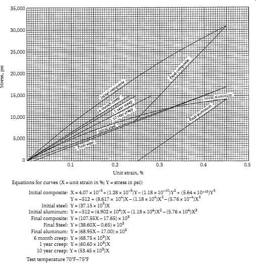
FIG. 8 is a stress-strain curve (Aluminum Association, 1974) for an all-aluminum 37-strand conductor ranging in size from 250 to 1033.5 kcmil. Because the conductor is made entirely of aluminum, there is only one initial and final curve.
3.1.1 Permanent Elongation
Once a conductor has been installed at an initial tension, it can elongate further. Such elongation results from two phenomena: permanent elongation due to high tension levels resulting from ice and wind loads, and creep elongation under everyday tension levels. These types of conductor elongation are discussed in the following sections.
3.1.2 Permanent Elongation due to Heavy Loading
Both Figures 15.7 and 15.8 indicate that when the conductor is initially installed, it elongates following the initial curve that is not a straight line. If the conductor tension increases to a relatively high level under ice and wind loading, the conductor will elongate. When the wind and ice loads abate, the conductor elongation will reduce along a curve parallel to the final curve, but the conductor will never return to its original length.
For example, refer to FIG. 8 and assume that a newly strung 795 kcmil-37 strand AAC "Arbutus" conductor has an everyday tension of 2780 lb. The conductor area is 0.6245 in. 2 , so the everyday stress is 4450 psi and the elongation is 0.062%. Following an extremely heavy ice and wind load event, assume that the conductor stress reaches 18,000 psi. When the conductor tension decreases back to everyday levels, the conductor elongation will be permanently increased by more than 0.2%. Also the sag under everyday conditions will be correspondingly higher, and the tension will be less. In most numerical sag-tension methods, final sag-tensions are calculated for such permanent elongation due to heavy loading conditions.
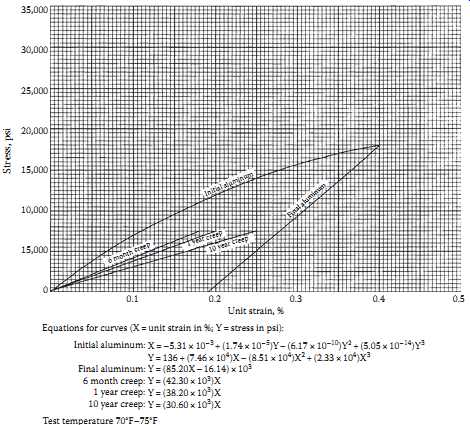
Above: Fig. 8 Stress-strain curves for 37-strand AAC.
3.1.3 Permanent Elongation at Everyday Tensions (Creep Elongation)
Conductors permanently elongate under tension even if the tension level never exceeds everyday levels.
This permanent elongation caused by everyday tension levels is called creep (Aluminum Company of America, 1961). Creep can be determined by long-term laboratory creep tests, the results of which are used to generate creep curves. On stress-strain graphs, creep curves are usually shown for 6 month, 1 year, and 10 year periods. FIG. 8 shows these typical creep curves for a 37 strand 250.0 through 1033.5 kcmil AAC. In FIG. 8, assume that the conductor tension remains constant at the initial stress of 4450 psi. At the intersection of this stress level and the initial elongation curve, 6 month, 1 year, and 10 year creep curves, the conductor elongation from the initial elongation of 0.062% increases to 0.11%, 0.12%, and 0.15%, respectively. Because of creep elongation, the resulting final sags are greater and the conductor tension is less than the initial values.
Creep elongation in aluminum conductors is quite predictable as a function of time and obeys a simple exponential relationship. Thus, the permanent elongation due to creep at everyday tension can be found for any period of time after initial installation. Creep elongation of copper and steel conductors is much less and is normally ignored.
Permanent increase in conductor length due to heavy load occurrences cannot be predicted at the time that a line is built. The reason for this unpredictability is that the occurrence of heavy ice and wind is random. A heavy ice storm may occur the day after the line is built or may never occur over the life of the line.
TBL. 4 Sag-Tension Data 795 kcmil-26/7 ACSR "Drake" with NESC Heavy Loading
TBL. 5 Tension Differences in Adjacent Dead-End Spans
3.2 Sag-Tension Tables
To illustrate the result of typical sag-tension calculations, refer to Tables 15.4 through 15.9 showing initial and final sag-tension data for 795 kcmil-26/7 ACSR "Drake," 795 kcmil-37 strand AAC "Arbutus," and 795 kcmil Type 16 "Drake/SDC" conductors in NESC light and heavy loading areas for spans of 1000 and 300 ft. Typical tension constraints of 15% final unloaded at 60°F, 25% initial unloaded at 60°F, and 60% initial at maximum loading are used.
With most sag-tension calculation methods, final sags are calculated for both heavy ice/wind load and for creep elongation. The final sag-tension values reported to the user are those with the greatest increase in sag.
TBL. 6 Sag and Tension Data for 795 kcmil-26/7 ACSR "Drake" 600 ft Ruling Span
Conductor: Drake 795 kcmil-26/7 ACSR Span = 600 ft Area = 0.7264 in. 2 Creep is not a factor NESC Heavy Loading District
3.2.1 Initial vs. Final Sags and Tensions
Rather than calculate the line sag as a function of time, most sag-tension calculations are determined based on initial and final loading conditions. Initial sags and tensions are simply the sags and tensions at the time the line is built. Final sags and tensions are calculated if (1) the specified ice and wind loading has occurred, and (2) the conductor has experienced 10 years of creep elongation at a conductor temperature of 60°F at the user-specified initial tension.
3.2.2 Special Aspects of ACSR Sag-Tension Calculations
Sag-tension calculations with ACSR conductors are more complex than such calculations with AAC, AAAC, or ACAR conductors. The complexity results from the different behavior of steel and aluminum strands in response to tension and temperature. Steel wires don’t exhibit creep elongation or plastic elongation in response to high tensions. Aluminum wires do creep and respond plastically to high stress levels. Also, they elongate twice as much as steel wires do in response to changes in temperature.
TBL. 10 presents various initial and final sag-tension values for a 600 ft span of a Drake ACSR conductor under heavy loading conditions. Note that the tension in the aluminum and steel components is shown separately. In particular, some other useful observations are as follows:
1. At 60°F, without ice or wind, the tension level in the aluminum strands decreases with time as the strands permanently elongate due to creep or heavy loading.
2. Both initially and finally, the tension level in the aluminum strands decreases with increasing temperature reaching zero tension at 212°F and 167°F for initial and final conditions, respectively.
3. At the highest temperature (212°F), where all the tension is in the steel core, the initial and final sag-tensions are nearly the same, illustrating that the steel core does not permanently elongate in response to time or high tension.
TBL. 8 Time-Sag Table for Stopwatch Method
TBL. 7 Stringing Sag Table for 795 kcmil-26/7 ACSR "Drake" 600 ft Ruling Span
TBL. 9 Sag-Tension Data 795 kcmil-26/7 ACSR "Drake" with NESC Light Loading 300 and 1000 ft Spans
TBL. 10 Sag-Tension Data 795 kcmil-26/7 ACSR "Drake" NESC Heavy Loading 300 and 1000 ft Spans
TBL. 11 Sag-Tension Data 795 kcmil-Type 16 ACSR/SD with NESC Light Loading 300 and 1000 ft Spans