Electric Machinery--Electromechanical-Energy-Conversion Principles

We are concerned here with the electromechanical-energy-conversion process, which takes place through the medium of the electric or magnetic field of the conversion device. Although the various conversion devices operate on similar principles, their structures depend on their function. Devices for measurement and control are frequently referred to as transducers; they generally operate under linear input-output conditions and with relatively small signals. The many examples include microphones, pickups, sensors, and loudspeakers. A second category of devices encompasses force-producing devices and includes solenoids, relays, and electromagnets. A third category includes continuous energy-conversion equipment such as motors and generators.

This section is devoted to the principles of electromechanical energy conversion and the analysis of the devices which accomplish this function. Emphasis is placed on the analysis of systems which use magnetic fields as the conversion medium since the remaining sections of the guide deal with such devices. However, the analytical techniques for electric field systems are quite similar.

The purpose of such analysis is threefold:

(1) to aid in understanding how energy conversion takes place, (2) to provide techniques for designing and optimizing the devices for specific requirements, and (3) to develop models of electromechanical energy-conversion devices that can be used in analyzing their performance as components in engineering systems. Transducers and force-producing devices are treated in this section; continuous energy-conversion devices are treated in the rest of the guide.

The concepts and techniques presented in this section are quite powerful and can be applied to a wide range of engineering situations involving electromechanical energy conversion. Sections 1 and 2 present a quantitative discussion of the forces in electromechanical systems and an overview of the energy method which forms the basis for the derivations presented here. Based upon the energy method, the remainder of the section develops expressions for forces and torques in magnetic-field-based electromechanical systems.

1. FORCES AND TORQUES IN MAGNETIC FIELD SYSTEMS

The Lorentz Force Law F = q(E + v × B) (EQN. 1)

gives the force F on a particle of charge q in the presence of electric and magnetic fields. In SI units, F is in newtons, q in coulombs, E in volts per meter, B in teslas, and v, which is the velocity of the particle relative to the magnetic field, in meters per second.

Thus, in a pure electric-field system, the force is determined simply by the charge on the particle and the electric field ...

F = qE (EQN. 2)

The force acts in the direction of the electric field and is independent of any particle motion.

In pure magnetic-field systems, the situation is somewhat more complex. Here the force ...

F = q(v × B) (EQN. 3)

is determined by the magnitude of the charge on the particle and the magnitude of the B field as well as the velocity of the particle. In fact, the direction of the force is always perpendicular to the direction of both the particle motion and that of the magnetic field. Mathematically, this is indicated by the vector cross product v × B in Eq. 3. The magnitude of this cross product is equal to the product of the magnitudes of v and B and the sine of the angle between them; its direction can be found from the fight-hand rule, which states that when the thumb of the fight hand points in the direction of v and the index finger points in the direction of B, the force, which is perpendicular to the directions of both B and v, points in the direction normal to the palm of the hand, as shown in FIG. 1.

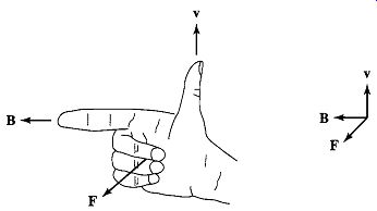
FIG. 1 Right-hand rule for determining the direction magnetic-field component of the Lorentz force F = q(v x B).

For situations where large numbers of charged particles are in motion, it is convenient to rewrite Eq. 1 in terms of the charge density p (measured in units of coulombs per cubic meter) as

Fv = p(E + v × B) (EQN. 4)

where the subscript v indicates that Fv is a force density (force per unit volume) which in SI units is measured in newtons per cubic meter.

The product p v is known as the current density

J = pv (EQN. 5)

which has the units of amperes per square meter. The magnetic-system force density corresponding to Eq. 3 can then be written as

Fv = J x B (EQN. 6)

For currents flowing in conducting media, Eq. 6 can be used to find the force density acting on the material itself. Note that a considerable amount of physics is hidden in this seemingly simple statement, since the mechanism by which the force is transferred from the moving charges to the conducting medium is a complex one.

For situations in which the forces act only on current-carrying elements and which are of simple geometry (such as that of Example 1), Eq. 6 is generally the simplest and easiest way to calculate the forces acting on the system. Unfortunately, very few practical situations fall into this class. In fact, as discussed in Section 1, most electromechanical-energy-conversion devices contain magnetic material; in these systems, forces act directly on the magnetic material and clearly cannot be calculated from Eq. 6.

Techniques for calculating the detailed, localized forces acting on magnetic materials are extremely complex and require detailed knowledge of the field distribution throughout the structure. Fortunately, most electromechanical-energy-conversion devices are constructed of rigid, non-deforming structures. The performance of these devices is typically determined by the net force, or torque, acting on the moving component, and it is rarely necessary to calculate the details of the internal force distribution. For example, in a properly designed motor, the motor characteristics are determined by the net accelerating torque acting on the rotor; accompanying forces, which act to squash or deform the rotor, play no significant role in the performance of the motor and generally are not calculated.

To understand the behavior of rotating machinery, a simple physical picture is quite useful. Associated with the rotor structure is a magnetic field (produced in many machines by currents in windings on the rotor), and similarly with the stator; one can picture them as a set of north and south magnetic poles associated with each structure. Just as a compass needle tries to align with the earth's magnetic field, these two sets of fields attempt to align, and torque is associated with their displacement from alignment. Thus, in a motor, the stator magnetic field rotates ahead of that of the rotor, pulling on it and performing work. The opposite is true for a generator, in which the rotor does the work on the stator.

Various techniques have evolved to calculate the net forces of concern in the electromechanical-energy-conversion process. The technique developed in this section and used throughout the guide is known as the energy method and is based on the principle of conservation of energy. The basis for this method can be understood with reference to FIG. 3a, where a magnetic-field-based electromechanical-energy-conversion device is indicated schematically as a lossless magnetic-energy-storage system with two terminals. The electric terminal has two terminal variables, a voltage e and a current i, and the mechanical terminal also has two terminal variables, a force ffld and a position x.

This sort of representation is valid in situations where the loss mechanism can be separated (at least conceptually) from the energy-storage mechanism. In these cases the electrical losses, such as ohmic losses in windings, can be represented as external elements (i.e., resistors) connected to the electric terminals, and the mechanical losses, such as friction and windage, can be included external to the mechanical terminals.

FIG. 3b shows an example of such a system; a simple force-producing device with a single coil forming the electric terminal, and a movable plunger serving as the mechanical terminal.

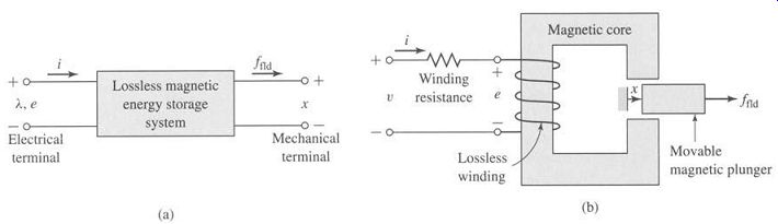
FIG. 3 (a) Schematic magnetic-field electromechanical-energy-conversion device; (b) simple force-producing device.

The interaction between the electric and mechanical terminals, i.e., the electromechanical energy conversion, occurs through the medium of the magnetic stored energy. Since the energy-storage system is lossless, it is a simple matter to write that the time rate of change of Wild, the stored energy in the magnetic field, is equal to the electric power input (given by the product of the terminal voltage and current) less the mechanical power output of the energy storage system (given by the product of the mechanical force and the mechanical velocity)"

(EQN. 7)

Recognizing that, from Eq. 27, the voltage at the terminals of our lossless winding is given by the time-derivative of the winding flux linkages

(EQN. 8)

dt and multiplying Eq. 7 by dt, we get:

(EQN. 9)

As shown in Section 4, Eq. 9 permits us to solve for the force simply as a function of the flux ~. and the mechanical terminal position x. Note that this result comes about as a consequence of our assumption that it is possible to separate the losses out of the physical problem, resulting in a lossless energy-storage system, as in FIG. 3a.

Equations 7 and 9 form the basis for the energy method. This technique is quite powerful in its ability to calculate forces and torques in complex electromechanical energy-conversion systems. The reader should recognize that this power comes at the expense of a detailed picture of the force-producing mechanism. The forces themselves are produced by such well-known physical phenomena as the Lorentz force on current carrying elements, described by Eq. 6, and the interaction of the magnetic fields with the dipoles in the magnetic material.

2. ENERGY BALANCE

The principle of conservation of energy states that energy is neither created nor destroyed; it is merely changed in form. For example, a golf ball leaves the tee with a certain amount of kinetic energy; this energy is eventually dissipated as heat due to air friction or rolling friction by the time the ball comes to rest on the fairway. Similarly, the kinetic energy of a hammer is eventually dissipated as heat as a nail is driven into a piece of wood. For isolated systems with clearly identifiable boundaries, this fact permits us to keep track of energy in a simple fashion: the net flow of energy into the system across its boundary is equal to the sum of the time rate of change of energy stored in the system.

This result, which is a statement of the first law of thermodynamics, is quite general. We apply it in this section to electromechanical systems whose predominant energy-storage mechanism is in magnetic fields. In such systems, one can account for [...]

Combining Eqs. 11 and 12 results in

… (EQN. 13)

Equation 3.13, together with Faraday's law for induced voltage (Eq. 1.27), form the basis for the energy method; the following sections illustrate its use in the analysis of electromechanical-energy-conversion devices.

3 ENERGY IN SINGLY-EXCITED MAGNETIC FIELD SYSTEMS

In Sections 1 and 2 we were concerned primarily with fixed-geometry magnetic circuits such as those used for transformers and inductors. Energy in those devices is stored in the leakage fields and to some extent in the core itself. However, the stored energy does not enter directly into the transformation process. In this section we are dealing with energy-conversion systems; the magnetic circuits have air gaps between the stationary and moving members in which considerable energy is stored in the magnetic field. This field acts as the energy-conversion medium, and its energy is the reservoir between the electric and mechanical systems.

Consider the electromagnetic relay shown schematically in FIG. 4. The resistance of the excitation coil is shown as an external resistance R, and the mechanical terminal variables are shown as a force fnd produced by the magnetic field directed from the relay to the external mechanical system and a displacement x; mechanical losses can be included as external elements connected to the mechanical terminal.

Similarly, the moving armature is shown as being massless; its mass represents mechanical energy storage and can be included as an external mass connected to the mechanical terminal. As a result, the magnetic core and armature constitute a lossless magnetic-energy-storage system, as is represented schematically in FIG. 3a.

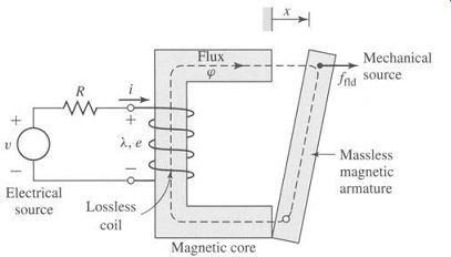
FIG. 4 Schematic of an electromagnetic relay.

This relay structure is essentially the same as the magnetic structures analyzed in Section 1. In Section 1 we saw that the magnetic circuit of FIG. 4 can be described by an inductance L which is a function of the geometry of the magnetic structure and the permeability of the magnetic material. Electromechanical-energy-conversion devices contain air gaps in their magnetic circuits to separate the moving parts. As discussed in Section 1.1, in most such cases the reluctance of the air gap is much larger than that of the magnetic material. Thus the predominant energy storage occurs in the air gap, and the properties of the magnetic circuit are determined by the dimensions of the air gap.

Because of the simplicity of the resulting relations, magnetic nonlinearity and core losses are often neglected in the analysis of practical devices. The final results of such approximate analyses can, if necessary, be corrected for the effects of these neglected factors by semi-empirical methods. Consequently, analyses are carried out under the assumption that the flux and mmf are directly proportional for the entire magnetic circuit. Thus the flux linkages ~. and current i are considered to be linearly related by an inductance which depends solely on the geometry and hence on the armature position x.

(EQN. 14)

where the explicit dependence of L on x has been indicated.

Since the magnetic force ftd has been defined as acting from the relay upon the external mechanical system and d Wmech is defined as the mechanical energy output of the relay, we can write

(EQN. 15)

Thus, using Eq. 15 and the substitution

[…]

we can write Eq. 11 as

(EQN. 16)

Since the magnetic energy storage system is lossless, it is a conservative system and the value of Wild is uniquely specified by the values of Z and x; ~. and x are thus referred to as state variables since their values uniquely determine the state of the system.

FIG. 5 Integration paths for ~ld.

From this discussion we see that Wild, being uniquely determined by the values of ~ and x, is the same regardless of how )~ and x are brought to their final values.

Consider FIG. 5, in which two separate paths are shown over which Eq. 16 can be integrated to find Wild at the point (~.0, x0). Path 1 is the general case and is difficult to integrate unless both i and fnd are known explicitly as a function of)~ and x. However, because the integration of Eq. 16 is path independent, path 2 gives the same result and is much easier to integrate. From Eq. 16

(EQN. 17)

path 2a path 2b

Notice that on path 2a, d)~ = 0 and ffld "-0 (since ~. = 0 and there can be no magnetic force in the absence of magnetic fields). Thus from Eq. 16, d Wfld = 0 on path 2a.

On path 2b, dx = 0, and, thus, from Eq. 16, Eq. 17 reduces to the integral of i d)~ over path 2b (for which x = x0).

(EQN. 18)

For a linear system in which )~ is proportional to i, as in Eq. 14, Eq. 18 gives:

(EQN. 19)

It can be shown that the magnetic stored energy can also be expressed in terms of the energy density of the magnetic field integrated over the volume V of the magnetic field. In this case (J0") Wild : H. dB' dV (EQN. 20)

For soft magnetic material of constant permeability (B =/zH), this reduces to ...

(EQN. 21)

4. DETERMINATION OF MAGNETIC FORCE AND TORQUE FROM ENERGY

As discussed in Section 3, for a lossless magnetic-energy-storage system, the magnetic stored energy Wild is a state function, determined uniquely by the values of the independent state variables ~. and x. This can be shown explicitly by rewriting Eq. 16 in the form

(EQN. 22)

For any state function of two independent variables, e.g., F(Xl, x2), the total differential of F with respect to the two state variables X l and x2 can be written ...

(EQN. 23)

It is extremely important to recognize that the partial derivatives in Eq. 23 are each taken by holding the opposite state variable constant.

Equation 3.23 is valid for any state function F and hence it is certainly valid for Wnd; thus ...

(EQN. 24)

Since k and x are independent variables, Eqs. 3.22 and 3.24 must be equal for all values of d~ and dx, and so ...

(EQN. 25)

where the partial derivative is taken while holding x constant and

(EQN. 26)

...in this case holding )~ constant while taking the partial derivative.

This is the result we have been seeking. Once we know Wild as a function of )~ and x, Eq. 25 can be used to solve for i (~., x). More importantly, Eq. 26 can be used to solve for the mechanical force ffld (~, x). It cannot be overemphasized that the partial derivative of Eq. 26 is taken while holding the flux linkages ~. constant. This is easily done provided W~d is a known function of ~. and x. Note that this is purely a mathematical requirement and has nothing to do with whether Z is held constant when operating the actual device.

The force ffld is determined from Eq. 26 directly in terms of the electrical state variable ~.. If we then want to express the force as a function of i, we can do so by substituting the appropriate expression for ~. as a function of i into the expression for fna that is obtained by using Eq. 26.

For linear magnetic systems for which ~. = L(x)i, the energy is expressed by Eq. 19 and the force can be found by direct substitution in Eq. 26

(EQN. 27)

If desired, the force can now be expressed in directly in terms of the current i simply by substitution of ~. -L(x)i

(EQN. 28)

5. DETERMINATION OF MAGNETIC FORCE AND TORQUE FROM COENERGY

A mathematical manipulation of Eq. 22 can be used to define a new state function, known as the coenergy, from which the force can be obtained directly as a function of the current. The selection of energy or coenergy as the state function is purely a matter of convenience; they both give the same result, but one or the other may be simpler analytically, depending on the desired result and the characteristics of the system being analyzed.

The coenergy W~d is defined as a function of i and x such that ...

(EQN. 34)

(EQN. 35)

(EQN. 36)

(EQN. 37)

(EQN. 38)

(EQN. 39)

(EQN. 40)

Equation 40 gives the mechanical force directly in terms of i and x. Note that the partial derivative in Eq. 40 is taken while homing i constant; thus W~d must be a known function of i and x. For any given system, Eqs. 26 and 40 will give the same result; the choice as to which to use to calculate the force is dictated by user preference and convenience.

By analogy to the derivation of Eq. 18, the coenergy can be found from the integral of ~. di

(EQN. 41)

For linear magnetic systems for which ~. = L(x)i, the co-energy is therefore given by ...

(EQN. 42)

(EQN. 43)

... which, as expected, is identical to the expression given by Eq. 28.

Similarly, for a system with a rotating mechanical displacement, the co-energy can be expressed in terms of the current and the angular displacement 0

(EQN. 44)

(EQN. 45)

(EQN. 46)

(EQN. 47)

which is identical to Eq. 33.

In field-theory terms, for soft magnetic materials (for which B = 0 when H = 0), it can be shown that...

(EQN. 48)

For soft magnetic material with constant permeability (B =/zH), this reduces to ...

(EQN. 49)

For permanent-magnet (hard) materials such as those which are discussed in Section 1 and for which B = 0 when H = Hc, the energy and coenergy are equal to zero when B = 0 and hence when H = Hc. Thus, although Eq. 20 still applies for calculating the energy, Eq. 48 must be modified to the form ...

(EQN. 50)

Note that Eq. 50 can be considered to apply in general since soft magnetic materials can be considered to be simply hard magnetic materials with Hc -0, in which case Eq. 50 reduces to Eq. 48.

In some cases, magnetic circuit representations may be difficult to realize or may not yield solutions of the desired accuracy. Often such situations are characterized by complex geometries and/or magnetic materials driven deeply into saturation. In such situations, numerical techniques can be used to evaluate the system energy using Eq. 20 or the coenergy using either Eqs. 3.48 or 3.50. One such technique, known as the finite-element method, 1 has become widely used. For example, such programs, which are available commercially from a number of vendors, can be used to calculate the system coenergy for various values of the displacement x of a linear-displacement actuator (making sure to hold the current constant as x is varied). The force can then be obtained from Eq. 40, with the derivative of coenergy with respect to x being calculated numerically from the results of the finite-element analysis.

For a magnetically-linear system, the energy and coenergy are numerically equal:

The same is true for the energy and coenergy densities" g/zl H 2. For a nonlinear system in which X and i or B and H are not linearly proportional, the two functions are not even numerically equal. A graphical interpretation of the energy and coenergy for a nonlinear system is shown in FIG. 10. The area between the ~. i curve and the vertical axis, equal to the integral of i dX, is the energy. The area to the horizontal axis given by the integral of X di is the coenergy.

For this singly-excited system, the sum of the energy and coenergy is, by definition (see Eq. 34), ...

(EQN. 51)

The force produced by the magnetic field in a device such as that of FIG. 4 for some particular value of x and i or X cannot, of course, depend upon whether it is calculated from the energy or coenergy. A graphical illustration will demonstrate that both methods must give the same result.

Assume that the relay armature of FIG. 4 is at position x so that the device is operating at point a in FIG. 11 a. The partial derivative of Eq. 26 can be interpreted as the limit of A Wild~ Ax with X constant as Ax --+ 0. If we allow a change Ax, the change -A Wad is shown by the shaded area in FIG. 11a. Hence, the force fad = (shaded area)/Ax as Ax --+ 0. On the other hand, the partial derivative of Eq. 40 can be interpreted as the limit of A W~d /Ax with i constant as Ax --+ 0. This perturbation of the device is shown in FIG. 11b; the force fad = (shaded area)/Ax as Ax --+ 0.

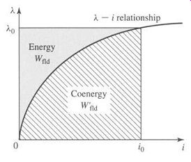
FIG. 10 Graphical interpretation of energy and coenergy in a singly-excited system.

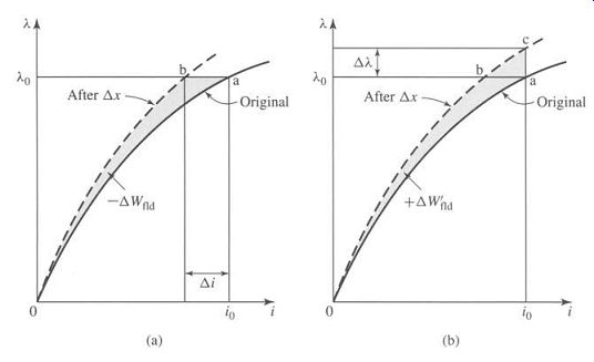
FIG. 11 Effect of Ax on the energy and coenergy of a singly-excited device: (a) change of energy with k held constant; (b) change of coenergy with i held constant.

The shaded areas differ only by the small triangle abc of sides Ai and AX, so that in the limit the shaded areas resulting from Ax at constant X or at constant i are equal. Thus the force produced by the magnetic field is independent of whether the determination is made with energy or coenergy.

Equations 26 and 40 express the mechanical force of electrical origin in terms of partial derivatives of the energy and coenergy functions Wild(k, x) and W~d(i, x). It is important to note two things about them: the variables in terms of which they must be expressed and their algebraic signs. Physically, of course, the force depends on the dimension x and the magnetic field. The field (and hence the energy or coenergy)

can be specified in terms of flux linkage k, or current i, or related variables. We again emphasize that the selection of the energy or coenergy function as a basis for analysis is a matter of convenience.

The algebraic signs in Eqs. 3.26 and 3.40 show that the force acts in a direction to decrease the magnetic field stored energy at constant flux or to increase the coenergy at constant current. In a singly-excited device, the force acts to increase the inductance by pulling on members so as to reduce the reluctance of the magnetic path linking the winding.

6. MULTIPLY-EXCITED MAGNETIC FIELD SYSTEMS

Many electromechanical devices have multiple electrical terminals. In measurement systems it is often desirable to obtain torques proportional to two electric signals; a meter which determines power as the product of voltage and current is one example.

Similarly, most electromechanical-energy-conversion devices consist of multiply-excited magnetic field systems.

Analysis of these systems follows directly from the techniques discussed in previous sections. This section illustrates these techniques based on a system with two electric terminals. A schematic representation of a simple system with two electrical terminals and one mechanical terminal is shown in FIG. 13. In this case it represents a system with rotary motion, and the mechanical terminal variables are torque Tnd and angular displacement 0. Since there are three terminals, the system must be described in terms of three independent variables; these can be the mechanical angle 0 along with the flux linkages X1 and X2, currents i l and i2, or a hybrid set including one current and one flux.

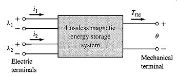
FIG. 13 Multiply-excited magnetic energy storage system.

When the fluxes are used, the differential energy function dWnd(~.l, X2, 0) corresponding to Eq. 29 is ...

(EQN. 52)

...and in direct analogy to the previous development for a singly-excited system ...

(EQN. 53)

(EQN. 54)

(EQN. 55)

Note that in each of these equations, the partial derivative with respect to each independent variable must be taken holding the other two independent variables constant.

The energy Wild can be found by integrating Eq. 52. As in the singly-excited case, this is most conveniently done by holding ~,1 and ~,2 fixed at zero and integrating first over 0; under these conditions, Tnd is zero, and thus this integral is zero. One can then integrate over ,k2 (while holding ~1 zero) and finally over ~.1. Thus:

(EQN. 56)

This path of integration is illustrated in FIG. 14 and is directly analogous to that of FIG. 5. One could, of course, interchange the order of integration for ~.2 and ~.1. It is extremely important to recognize, however, that the state variables are integrated over a specific path over which only one state variable is varied at a time; for example, ~.1 is maintained at zero while integrating over ~2 in Eq. 56. This is explicitly indicated in Eq. 56 and can also be seen from FIG. 14. Failure to observe this requirement is one of the most common errors made in analyzing these systems.

In a magnetically-linear system, the relationships between)~ and i can be specified in terms of inductances as is discussed in Section 1.2

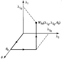
FIG. 14 Integration path to obtain ~ld(Z.10, Z.2o, eo).

(EQN. 57)

(EQN. 58)

where

(EQN. 59)

Here the inductances are, in general, functions of angular position 0. These equations can be inverted to obtain expressions for the i's as a function of the 0's

(EQN. 60)

(EQN. 61)

(EQN. 62)

The energy for this linear system can be found from Eq. 56 ....

...where the dependence of the inductances and the determinant D(O) on the angular displacement 0 has been explicitly indicated.

In Section 5, the coenergy function was defined to permit determination of force and torque directly in terms of the current for a single-winding system. A similar coenergy function can be defined in the case of systems with two windings as ...

(EQN. 64)

It is a state function of the two terminal currents and the mechanical displacement.

Its differential, following substitution of Eq. 52, is given by:

(EQN. 65)

(EQN. 66)

(EQN. 67)

Most significantly, the torque can now be determined directly in terms of the currents as

(EQN. 68)

Analogous to Eq. 56, the coenergy can be found as:

(EQN. 70)

(EQN. 69)

For such a linear system, the torque can be found either from the energy of Eq. 63 using Eq. 55 or from the coenergy of Eq. 70 using Eq. 68. It is at this point that the utility of the coenergy function becomes apparent. The energy expression of Eq. 63 is a complex function of displacement, and its derivative is even more so. Alternatively, the coenergy function is a relatively simple function of displacement, and from its derivative a straightforward expression for torque can be determined as a function of the winding currents i1 and i2 as ...

(EQN. 71)

Systems with more than two electrical terminals are handled in analogous fashion.

As with the two-terminal-pair system above, the use of a coenergy function of the terminal currents greatly simplifies the determination of torque or force.

7. FORCES AND TORQUES IN SYSTEMS WITH PERMANENT MAGNETS

The derivations of the force and torque expressions of Sections 4 through 6 focus on systems in which the magnetic fields are produced by the electrical excitation of specific windings in the system. However, in Section 5, it is seen that special care must be taken when considering systems which contain permanent magnets (also referred to as hard magnetic materials). Specifically, the discussion associated with the derivation of the coenergy expression of Eq. 50 points out that in such systems the magnetic flux density is zero when H = Hc, not when H = 0. For this reason, the derivation of the expressions for force and torque in Sections 4 through 6 must be modified for systems which contain permanent magnets. Consider for example that the derivation of Eq. 18 depends on the fact that in Eq. 17 the force can be assumed zero when integrating over path 2a because there is no electrical excitation in the system. A similar argument applies in the derivation of the coenergy expressions of Eqs. 41 and 69.

In systems with permanent magnets, these derivations must be carefully revisited.

In some cases, such systems have no windings at all, their magnetic fields are due solely to the presence of permanent-magnet material, and it is not possible to base a derivation purely upon winding fluxes and currents. In other cases, magnetic fields may be produced by a combination of permanent magnets and windings.

A modification of the techniques presented in the previous sections can be used in systems which contain permanent magnets. Although the derivation presented here applies specifically to systems in which the magnet appears as an element of a magnetic circuit with a uniform internal field, it can be generalized to more complex situations; in the most general case, the field theory expressions for energy (Eq. 20) and coenergy (Eq. 50) can be used.

The essence of this technique is to consider the system as having an additional fictitious winding acting upon the same portion of the magnetic circuit as does the permanent magnet. Under normal operating conditions, the fictitious winding carries zero current. Its function is simply that of a mathematical "crutch" which can be used to accomplish the required analysis. The current in this winding can be adjusted to zero-out the magnetic fields produced by the permanent magnet in order to achieve the "zero-force" starting point for the analyses such as that leading from Eq. 17 to Eq. 18.

For the purpose of calculating the energy and coenergy of the system, this winding is treated as any other winding, with its own set of current and flux linkages. As a result, energy and coenergy expressions can be obtained as a function of all the winding flux linkages or currents, including those of the fictitious winding. Since under normal operating conditions the current in this winding will be set equal to zero, it is useful to derive the expression for the force from the system coenergy since the winding currents are explicitly expressed in this representation.

FIG. 17a shows a magnetic circuit with a permanent magnet and a movable plunger. To find the force on the plunger as a function of the plunger position, we assume that there is a fictitious winding of Nf turns carrying a current if wound so as to produce flux through the permanent magnet, as shown in FIG. 17b.

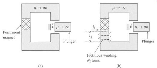
FIG. 17 (a) Magnetic circuit with permanent magnet and movable plunger; (b) fictitious winding added.

For this single-winding system we can write the expression for the differential in coenergy from Eq. 37 as ...

(EQN. 78)

...where the subscript 'f' indicates the fictitious winding. Corresponding to Eq. 40, the force in this system can be written as ...

(EQN. 79)

...where the partial derivative is taken while holding if constant, and the resultant expression is then evaluated at if = 0, which is equivalent to setting if--0 in the expression for W~o before taking the derivative. As we have seen, holding if constant for the derivative in Eq. 79 is a requirement of the energy method; it must be set to zero to properly calculate the force due to the magnet alone so as not to include a force component from current in the fictitious winding.

To calculate the coenergy W~d(if, x) in this system, it is necessary to integrate Eq. 78. Since W~d is a state function of if and x, we are free to choose any integration path we wish. FIG. 18 illustrates a path over which this integration is particularly simple. For this path we can write the expression for coenergy in this system as:

(EQN. 80)

....which corresponds directly to the analogous expression for energy found in Eq. 17.

Note that the integration is initially over x with the current if held fixed at if ---If0.

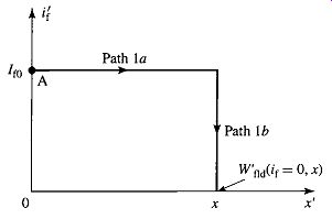
FIG. 18 Integration path for calculating Wild(if -O, X) in the permanent magnet system of FIG. 17.

This is a very specific current, equal to that fictitious-winding current which reduces the magnetic flux in the system to zero. In other words, the current If0 is that current in the fictitious winding which totally counteracts the magnetic field produced by the permanent magnet. Thus, the force ffld is zero at point A in FIG. 18 and remains so for the integral over x of path la. Hence the integral over path la in Eq. 80 is zero, and Eq. 80 reduces to

(EQN. 81)

Note that Eq. 81 is perfectly general and does not require either the permanent magnet or the magnetic material in the magnetic circuit to be linear. Once Eq. 81 has been evaluated, the force at a given plunger position x can be readily found from Eq. 79. Note also that due to the presence of the permanent magnet, neither the coenergy nor the force is zero when if is zero, as we would expect.

Consider the schematic magnetic circuit of FIG. 21 a. It consists of a section of linear, hard magnetic material (Bm = krR(Hm -Hc~)) of area A and length d. It is connected in series with an external magnetic circuit of mmf f'e.

From Eq. 1.21, since there are no ampere-turns acting on this magnetic circuit, ...

(EQN. 82)

The flux produced in the external magnetic circuit by the permanent magnet is given by ...

(EQN. 83)

(EQN. 84)

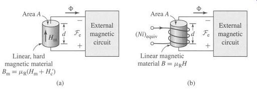
FIG. 21 (a) Generic magnetic circuit containing a section of linear, permanent-magnet material. (b) Generic magnetic circuit in which the permanent-magnet material has been replaced by a section of linear magnetic material and a fictitious winding.

Now consider the schematic magnetic circuit of FIG. 21b in which the linear, hard magnetic material of FIG. 21a has been replaced by soft, linear magnetic material of the same permeability (B = #RH) and of the same dimensions, length d and area A. In addition, a winding carrying (Ni)equiv ampere-turns has been included.

For this magnetic circuit, the flux can be shown to be given by ...

(EQN. 85)

Comparing Eqs. 84 and 85, we see that the same flux is produced in the external magnetic circuit if the ampere-turns, (Ni)equiv, in the winding of FIG. 21b is equal to -ncd.

This is a useful result for analyzing magnetic-circuit structures which contain linear, permanent-magnet materials whose B-H characteristic can be represented in the form of Eq. 1.61. In such cases, replacing the permanent-magnet section with a section of linear-magnetic material of the same permeability #R and geometry and an equivalent winding of ampere-turns:

(EQN. 86)

results in the same flux in the external magnetic circuit. As a result, both the linear permanent magnet and the combination of the linear magnetic material and the winding are indistinguishable with regard to the production of magnetic fields in the external magnetic circuit, and hence they produce identical forces. Thus, the analysis of such systems may be simplified by this substitution, as is shown in Example 9.

This technique is especially useful in the analysis of magnetic circuits containing both a permanent magnetic and one or more windings.

Clearly the methods described in this section can be extended to handle situations in which there are permanent magnets and multiple current-carrying windings. In many devices of practical interest, the geometry is sufficiently complex, independent of the number of windings and/or permanent magnets, that magnetic-circuit analysis is not necessarily applicable, and analytical solutions can be expected to be inaccurate, if they can be found at all. In these cases, numerical techniques, such as the finite-element method discussed previously, can be employed. Using this method, the coenergy of Eq. 48, or Eq. 50 if permanent magnets are involved, can be evaluated numerically at constant winding currents and for varying values of displacement.

8. DYNAMIC EQUATIONS

We have derived expressions for the forces and torques produced in electromechanical energy-conversion devices as functions of electrical terminal variables and mechanical displacement. These expressions were derived for conservative energy-conversion systems for which it can be assumed that losses can be assigned to external electrical and mechanical elements connected to the terminals of the energy-conversion system.

Such energy-conversion devices are intended to operate as a coupling means between electric and mechanical systems. Hence, we are ultimately interested in the operation of the complete electromechanical system and not just of the electromechanical energy-conversion system around which it is built.

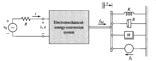
FIG. 23 Model of a singly-excited electromechanical system.

The model of a simple electro-mechanical system shown in FIG. 23 shows the basic system components, the details of which may vary from system to system. The system shown consists of three parts: an external electric system, the electromechanical energy-conversion system, and an external mechanical system. The electric system is represented by a voltage source v0 and resistance R; the source could alternatively be represented by a current source and a parallel conductance G. Note that all the electrical losses in the system, including those which are inherent to the electromechanical-energy-conversion system are assigned to the resistance R in this model. For example, if the voltage source has an equivalent resistance Rs and the winding resistance of the electromechanical-energy-conversion system is Rw, the resistance R would equal the sum of these two resistances; R = Rs + Rw.

The electric equation for this model is...

(EQN. 87)

...dt If the flux linkage ~. can be expressed as ~. = L (x)i, the external equation becomes...

(EQN. 88)

The second term on the fight, L(di/dt), is the self-inductance voltage term. The third term i(dL/dx)(dx/dt) includes the multiplier dx/dt. This is the speed of the mechanical terminal, and the third term is often called simply the speed voltage.

The speed-voltage term is common to all electromechanical-energy-conversion systems and is responsible for energy transfer to and from the mechanical system by the electrical system.

For a multiply-excited system, electric equations corresponding to Eq. 87 are written for each input pair. If the expressions for the )~'s are to be expanded in terms of inductances, as in Eq. 88, both self- and mutual-inductance terms will be required.

The mechanical system of FIG. 23 includes the representation for a spring (spring constant K), a damper (damping constant B), a mass M, and an external mechanical excitation force f0. Here, as for the electrical system, the damper represents the losses both of the external mechanical system as well as any mechanical losses of the electromechanical-energy-conversion system.

The x-directed forces and displacement x are related as follows:

Spring: Damper: Mass:

(EQN. 89)

(EQN. 90)

(EQN. 91)

where x0 is the value of x with the spring normally unstretched. Force equilibrium thus requires that

(EQN. 92)

Combining Eqs. 3.88 and 3.92, the differential equations for the overall system of FIG. 23 for arbitrary inputs vo(t) and fo(t) are thus

(EQN. 93)

(EQN. 94)

The functions L (x) and ffld (X, i) depend on the properties of the electromechanical energy-conversion system and are calculated as previously discussed.

9. ANALYTICAL TECHNIQUES

We have described relatively simple devices in this section. The devices have one or two electrical terminals and one mechanical terminal, which is usually constrained to incremental motion. More complicated devices capable of continuous energy conversion are treated in the following sections. The analytical techniques discussed here apply to the simple devices, but the principles are applicable to the more complicated devices as well.

Some of the devices described in this section are used to produce gross motion, such as in relays and solenoids, where the devices operate under essentially "on" and "off" conditions. Analysis of these devices is carried out to determine force as a function of displacement and reaction on the electric source. Such calculations have already been made in this section. If the details of the motion are required, such as the displacement as a function of time after the device is energized, nonlinear differential equations of the form of Eqs. 3.93 and 3.94 must be solved.

In contrast to gross-motion devices, other devices such as loudspeakers, pickups, and transducers of various kinds are intended to operate with relatively small displacements and to produce a linear relationship between electrical signals and mechanical motion, and vice versa. The relationship between the electrical and mechanical variables is made linear either by the design of the device or by restricting the excursion of the signals to a linear range. In either case the differential equations are linear and can be solved using standard techniques for transient response, frequency response, and so forth, as required.

9.1 Gross Motion

The differential equations for a singly-excited device as derived in Example 10 are of the form:

(EQN. 95)

(EQN. 96)

A typical problem using these differential equations is to find the excursion x(t)

when a prescribed voltage vt = V0 is applied at t = 0. An even simpler problem is to find the time required for the armature to move from its position x (0) at t = 0 to a given displacement x = X when a voltage vt -V is applied at t = 0. There is no general analytical solution for these differential equations; they are nonlinear, involving products and powers of the variables x and i and their derivatives. They can be solved using computer-based numerical integration techniques.

In many cases the gross-motion problem can be simplified and a solution found by relatively simple methods. For example, when the winding of the device is connected to the voltage source with a relatively large resistance, the i R term dominates on the fight-hand side of Eq. 96 compared with the di/dt self-inductance voltage term and the dx/dt speed-voltage term. The current i can then be assumed equal to V/R and inserted directly into Eq. 95. The same assumption can be made when the winding is driven from power electronic circuitry which directly controls the current to the winding. With the assumption that i = V/R, two cases can be solved easily.

Case 1 The first case includes those devices in which the dynamic motion is dominated by damping rather than inertia, e.g., devices purposely having low inertia or relays having dashpots or dampers to slow down the motion. For example, under such conditions, with j~ = 0, the differential equation of Eq. 95 reduces to

(EQN. 97)

where f (x) is the difference between the force of electrical origin and the spring force in the device of FIG. 24. The velocity at any value of x is merely dx/dt = f(x)/B; the time t to reach x = X is given by

(EQN. 98)

The integration of Eq. 98 can be carried out analytically or numerically.

Case 2 In this case, the dynamic motion is governed by the inertia rather than the damping. Again with j~ = 0, the differential equation of Eq. 95 reduces to:

(EQN. 99)

(EQN. 100)

(EQN. 101)

The integration of Eq. 101 can be carried out analytically or numerically to find v(x) and to find the time t to reach any value of x.

9.2 Linearization

Devices characterized by nonlinear differential equations such as Eqs. 95 and 96 will yield nonlinear responses to input signals when used as transducers. To obtain linear behavior, such devices must be restricted to small excursions of displacement and electrical signals about their equilibrium values. The equilibrium displacement is determined either by a bias mmf produced by a dc winding current, or a permanent magnet acting against a spring, or by a pair of windings producing mmf's whose forces cancel at the equilibrium point. The equilibrium point must be stable; the transducer following a small disturbance should return to the equilibrium position.

With the current and applied force set equal to their equilibrium values, 10 and f to respectively, the equilibrium displacement X0 and voltage V0 can be determined for the system described by Eqs. 95 and 96 by setting the time derivatives equal to zero. Thus

(EQN. 102)

(EQN. 103)

The incremental operation can be described by expressing each variable as the sum of its equilibrium and incremental values; thus i = Io + i', ft = fto + f', vt = V0 + v', and x = X0 + x'. The equations are then linearized by canceling any products of increments as being of second order. Equations 95 and 96 thus become

(EQN. 104)

(EQN. 105)

The equilibrium terms cancel, and retaining only first-order incremental terms yields a set of linear differential equations in terms of just the incremental variables of first order as

(EQN. 106)

(EQN. 107)

Standard techniques can be used to solve for the time response of this set of linear differential equations. Alternatively, sinusoidal-steady-state operation can be assumed, and Eqs. 3.106 and 3.107 can be converted to a set of linear, complex algebraic equations and solved in the frequency domain.

10. SUMMARY

In electromechanical systems, energy is stored in magnetic and electric fields. When the energy in the field is influenced by the configuration of the mechanical parts constituting the boundaries of the field, mechanical forces are created which tend to move the mechanical elements so that energy is transmitted from the field to the mechanical system.

Singly excited magnetic systems are considered first in Section 3. By removing electric and mechanical loss elements from the electromechanical-energy-conversion system (and incorporating them as loss elements in the external electrical and mechanical systems), the energy conversion device can be modeled as a conservative system. Its energy then becomes a state function, determined by its state variables ~. and x. Section 4 derives expressions for determining the force and torque as the negative of partial derivative of the energy with respect to the displacement, taken while holding the flux-linkage )~ constant.

In Section 5 the state function coenergy, with state variables i and x or 0, is introduced. The force and torque are then shown to be given by the partial derivative of the coenergy with respect to displacement, taken while holding the current i constant.

These concepts are extended in Section 6 to include systems with multiple windings. Section 7 further extends the development to include systems in which permanent magnets are included among the sources of the magnetic energy storage.

Energy conversion devices operate between electric and mechanical systems.

Their behavior is described by differential equations which include the coupling terms between the systems, as discussed in Section 8. These equations are usually nonlinear and can be solved by numerical methods if necessary. As discussed in Section 9, in some cases approximations can be made to simplify the equations.

For example, in many cases, linearized analyses can provide useful insight, both with respect to device design and performance.

This section has been concerned with basic principles applying broadly to the electromechanical-energy-conversion process, with emphasis on magnetic-field systems. Basically, rotating machines and linear-motion transducers work in the same way. The remainder of this text is devoted almost entirely to rotating machines.

Rotating machines typically include multiple windings and may include permanent magnets. Their performance can be analyzed by using the techniques and principles developed in this section.

11. PROBLEMS

1. The rotor of FIG. 25 is similar to that of FIG. 2 (Example 1) except that it has two coils instead of one. The rotor is nonmagnetic and is placed in a uniform magnetic field of magnitude B0. The coil sides are of radius R and are uniformly spaced around the rotor surface. The first coil is carrying a current 11 and the second coil is carrying a current 12.

Assuming that the rotor is 0.30 m long, R = 0.13 m, and B0 = 0.85 T, find the 0-directed torque as a function of rotor position ot for (a) 11 = 0 A and 12 = 5 A, (b) 11 = 5 A and 12 = 0 A, and (c) I1 = 8 A and I2 = 8 A.

2. The winding currents of the rotor of Problem 1 are controlled as a function of rotor angle ot such that: Ii=8sinot A and 12=8cosot A ]

Write an expression for the rotor torque as a function of the rotor position or.

3. Calculate the magnetic stored energy in the magnetic circuit of Example 1.2.

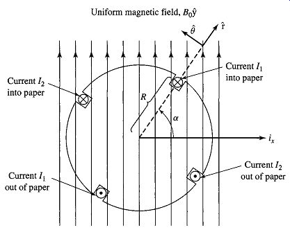
FIG. 25 Two-coil rotor for Problem 1.

4. An inductor has an inductance which is found experimentally to be of the form

2L0 L= 1 +x/xo

where L0 = 30 mH, x0 = 0.87 mm, and x is the displacement of a movable element. Its winding resistance is measured and found to equal 110 mr^2.

a. The displacement x is held constant at 0.90 mm, and the current is increased from 0 to 6.0 A. Find the resultant magnetic stored energy in the inductor.

b. The current is then held constant at 6.0 A, and the displacement is increased to 1.80 mm. Find the corresponding change in magnetic stored energy.

5. Repeat Problem 4, assuming that the inductor is connected to a voltage source which increases from 0 to 0.4 V (part [a]) and then is held constant at 0.4 V (part [b]). For both calculations, assume that all electric transients can be ignored.

6. The inductor of Problem 4 is driven by a sinusoidal current source of the form i (t) = Io sin cot where I0 = 5.5 A and 09 = 100n (50 Hz). With the displacement held fixed at x = x0, calculate (a) the time-averaged magnetic stored energy (Wild) in the inductor and (b) the time-averaged power dissipated in the winding resistance.

7. An actuator with a rotating vane is shown in FIG. 26. You may assume that the permeability of both the core and the vane are infinite (/z --+ oo). The total air-gap length is 2g and shape of the vane is such that the effective area of the air gap can be assumed to be of the form

Ag=Ao(1-('-~) 2)

(valid only in the range 101 _< Jr/6).

The actuator dimensions are g 0.8 mm, A0 = 6.0 mm^2, and N = 650 turns.

a. Assuming the coil to be carrying current i, write an expression for the magnetic stored energy in the actuator as a function of angle 0 for 101 _< rr/6.

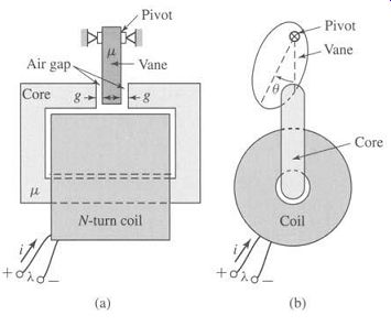
FIG. 26 Actuator with rotating vane for Problem 7. (a) Side view. (b) End view.

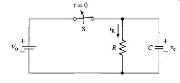
FIG. 27 An RC circuit for Problem 8.

b. Find the corresponding inductance L(O). Use MATLAB to plot this inductance as a function of 0. 3.8 An RC circuit is connected to a battery, as shown in FIG. 27. Switch S is initially closed and is opened at time t = 0.

a. Find the capacitor voltage vc(t) for t _> 0

b. What are the initial and final (t cxz) values of the stored energy in the capacitor?

(Hint: Wild 1 2 = ~ q /C, where q = C V0.)

What is the energy stored in the capacitor as a function of time?

c. What is the power dissipated in the resistor as a function of time? What is the total energy dissipated in the resistor? 3.9 An RL circuit is connected to a battery, as shown in FIG. 28. Switch S is initially closed and is opened at time t 0.

a. Find the inductor current iL(t) for t > 0. (Hint: Note that while the switch is closed, the diode is reverse-biased and can be assumed to be an open circuit. Immediately after the switch is opened, the diode becomes forward-biased and can be assumed to be a short circuit.)

b. What are the initial and final (t = c~) values of the stored energy in the inductor? What is the energy stored in the inductor as a function of time?

c. What is the power dissipated in the resistor as a function of time? What is the total energy dissipated in the resistor?

FIG. 28 An RL circuit for Problem 9.

10. The L/R time constant of the field winding of an 500-MVA synchronous generator is 4.8 s. At normal operating conditions, the field winding is known to be dissipating 1.3 MW. Calculate the corresponding magnetic stored energy.

FIG. 29 Plunger actuator for Problem 12.

11. The inductance of a phase winding of a three-phase salient-pole motor is measured to be of the form L( Om) = Lo + L2 cos 20m where 0m is the angular position of the rotor.

a. How many poles are on the rotor of this motor?

b. Assuming that all other winding currents are zero and that this phase is excited by a constant current I0, find the torque Tnd(0) acting on the rotor.

12 Cylindrical iron-clad solenoid actuators of the form shown in FIG. 29 are used for tripping circuit breakers, for operating valves, and in other applications in which a relatively large force is applied to a member which moves a relatively short distance. When the coil current is zero, the plunger drops against a stop such that the gap g is 2.25 cm. When the coil is energized by a direct current of sufficient magnitude, the plunger is raised until it hits another stop set so that g is 0.2 cm. The plunger is supported so that it can move freely in the vertical direction. The radial air gap between the shell and the plunger can be assumed to be uniform and 0.05 cm in length.

For this problem neglect the magnetic leakage and fringing in the air gaps. The exciting coil has 1300 turns and carries a constant current of 2.3 A. Assume that the mmf in the iron can be neglected and use MATLAB to:

a. plot the flux density in the variable gap between the yoke and the plunger for the range of travel of the plunger,

b. plot the corresponding values of the total energy stored in the magnetic field in/x J, and

c. plot the corresponding values of the coil inductance in #H. 3.13 Consider the plunger actuator of FIG. 29. Assume that the plunger is initially fully opened (g = 2.25 cm) and that a battery is used to supply a current of 2.5 A to the winding.

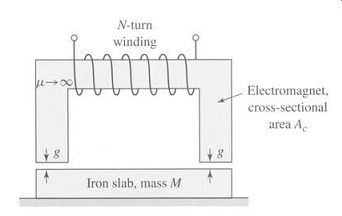
FIG. 30 Electromagnet lifting an iron slab (Problem 14).

a. If the plunger is constrained to move very slowly (i.e., slowly compared to the electrical time constant of the actuator), reducing the gap g from 2.25 to 0.20 cm, how much mechanical work in joules will be supplied to the plunger?

b. For the conditions of part (a), how much energy will be supplied by the battery (in excess of the power dissipated in the coil)?

14. As shown in FIG. 30, an N-turn electromagnet is to be used to lift a slab of iron of mass M. The surface roughness of the iron is such that when the iron and the electromagnet are in contact, there is a minimum air gap of g_min = 0.18 mm in each leg. The electromagnet cross-sectional area Ac = 32 cm and coil resistance is 2.8 f2. Calculate the minimum coil voltage which must be used to lift a slab of mass 95 kg against the force of gravity.

Neglect the reluctance of the iron.

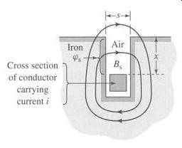
FIG. 31 Conductor in a slot (Problem 17).

15. Data for the magnetization curve of the iron portion of the magnetic circuit of the plunger actuator of Problem 12 are given below:

a. Use the MATLAB poly-fit function to obtain a 3'rd-order fit of reluctance and total flux versus mmf for the iron portions of the magnetic circuit.

Your fits will be of the form:

List the coefficients.

(i) Using MATLAB and the functional forms found in part (a), plot the magnetization curve for the complete magnetic circuit (flux linkages ), versus winding current i) for a variable-gap length of g = 0.2 cm. On the same axes, plot the magnetization curve corresponding to the assumption that the iron is of infinite permeability. The maximum current in your plot should correspond to a flux in the magnetic circuit of 600 mWb.

(ii) Calculate the magnetic field energy and coenergy for each of these cases corresponding to a winding current of 2.0 A.

c. Repeat part (b) for a variable-gap length of g = 2.25 cm. In part (ii), calculate the magnetic field energy and coenergy corresponding to a winding current of 20 A.

16. An inductor is made up of a 525-turn coil on a core of 14-cm^2 cross-sectional area and gap length 0.16 mm. The coil is connected directly to a 120-V 60-Hz voltage source. Neglect the coil resistance and leakage inductance. Assuming the coil reluctance to be negligible, calculate the time-averaged force acting on the core tending to close the air gap. How would this force vary if the air-gap length were doubled?

17. FIG. 31 shows the general nature of the slot-leakage flux produced by current i in a rectangular conductor embedded in a rectangular slot in iron.

Assume that the iron reluctance is negligible and that the slot leakage flux goes straight across the slot in the region between the top of the conductor and the top of the slot.

a. Derive an expression for the flux density Bs in the region between the top of the conductor and the top of the slot.

b. Derive an expression for the slot-leakage ~s sits crossing the slot above the conductor, in terms of the height x of the slot above the conductor, the slot width s, and the embedded length 1 perpendicular to the paper.

c. Derive an expression for the force f created by this magnetic field on a conductor of length 1. In what direction does this force act on the conductor?

d. When the conductor current is 850 A, compute the force per meter on a conductor in a slot 2.5 cm wide.

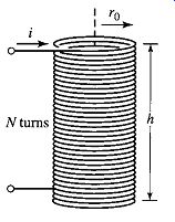
FIG. 32 Solenoid coil (Problem 18).

18. A long, thin solenoid of radius r0 and height h is shown in FIG. 32. The magnetic field inside such a solenoid is axially directed, essentially uniform and equal to H = N i/h. The magnetic field outside the solenoid can be shown to be negligible. Calculate the radial pressure in newtons per square meter acting on the sides of the solenoid for constant coil current i -I0.

19. An electromechanical system in which electric energy storage is in electric fields can be analyzed by techniques directly analogous to those derived in this section for magnetic field systems. Consider such a system in which it is possible to separate the loss mechanism mathematically from those of energy storage in electric fields. Then the system can be represented as in FIG. 33.

For a single electric terminal, Eq. 11 applies, where dWelec -vi dt = v dq where v is the electric terminal voltage and q is the net charge associated with electric energy storage. Thus, by analogy to Eq. 16, d Wnd = v dq fnd dx

a. Derive an expression for the electric stored energy Wild (q, x) analogous to that for the magnetic stored energy in Eq. 18.

b. Derive an expression for the force of electric origin ftd analogous to that of Eq. 26. State clearly which variable must be held constant when the derivative is taken.

c. By analogy to the derivation of Eqs. 34 to 41, derive an expression for the coenergy W~d(V , X) and the corresponding force of electric origin.

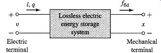
FIG. 33 Lossless electric energy storage system.

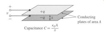
FIG. 34 Capacitor plates (Problem 20).

20. A capacitor (FIG. 34) is made of two conducting plates of area A separated in air by a spacing x. The terminal voltage is v, and the charge on the plates is q. The capacitance C, defined as the ratio of charge to voltage, is

q E0A C _._ _ 13 X

where E0 is the dielectric constant of free space (in SI units E0 = 8.85 X 10^-12 F/m).

a. Using the results of Problem 19, derive expressions for the energy Wild(q, x) and the coenergy W~d(V, x).

b. The terminals of the capacitor are connected to a source of constant voltage V0. Derive an expression for the force required to maintain the plates separated by a constant spacing x = 8.

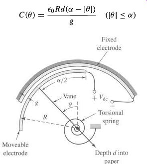
FIG. 35 Schematic electrostatic voltmeter (Problem 21).

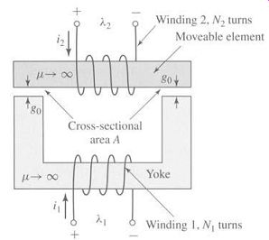
FIG. 36 Two-winding magnetic circuit for Problem 22.

21. FIG. 35 shows in schematic form an electrostatic voltmeter, a capacitive system consisting of a fixed electrode and a moveable electrode. The moveable electrode is connected to a vane which rotates on a pivot such that the air gap between the two electrodes remains fixed as the vane rotates. The capacitance of this system is given by

[…]

A torsional spring is connected to the moveable vane, producing a torque Tspring = -K (0 00) ...

a. For 0 _< 0 _< or, using the results of Problem 19, derive an expression for the electromagnetic torque Tnd in terms of the applied voltage Vdc.

b. Find an expression for the angular position of the moveable vane as a function of the applied voltage Vdc.

c. For a system with R -12 cm, d -4 cm, g -0.2 mm ot-zr/3rad, 00-0rad, K--3.65N.m/rad Plot the vane position in degrees as a function of applied voltage for ...

0 _< Vdc _< 1500 V.

22. The two-winding magnetic circuit of FIG. 36 has a winding on a fixed yoke and a second winding on a moveable element. The moveable element is constrained to motion such that the lengths of both air gaps remain equal.

a. Find the self-inductances of windings 1 and 2 in terms of the core dimensions and the number of turns.

b. Find the mutual inductance between the two windings.

c. Calculate the coenergy Wt~d(i1, i2).

d. Find an expression for the force acting on the moveable element as a function of the winding currents.

23. Two coils, one mounted on a stator and the other on a rotor, have self and mutual inductances of LI1 -3.5 mH L22 -1.8 mH L12 -2.1cos0 mH where 0 is the angle between the axes of the coils. The coils are connected in series and carry a current i = ~/-2I sin cot

a. Derive an expression for the instantaneous torque T on the rotor as a function of the angular position 0.

b. Find an expression for the time-averaged torque Tavg as a function of 0.

c. Compute the numerical value of Tavg for I -10 A and 0 = 90 °.

d. Sketch curves of Tavg versus 0 for currents I = 5, 7.07, and 10 A.

e. A helical restraining spring which tends to hold the rotor at 0 90 ° is now attached to the rotor. The restraining torque of the spring is proportional to the angular deflection from 0 -90 ° and is -0.1 N. m when the rotor is turned to 0 0 °. Show on the curves of part (d) how you could find the angular position of the rotor-plus-spring combination for coil currents I -5, 7.07, and 10 A. From your curves, estimate the rotor angle for each of these currents.

f. Write a MATLAB script to plot the angular position of the rotor as a function of rms current for 0 < I < 10 A. (Note that this problem illustrates the principles of the dynamometer-type ac ammeter.)

24. Two windings, one mounted on a stator and the other on a rotor, have self and mutual inductances of

LI1 4.5H L22 -2.5H L12 -2.8cos0 H

… where 0 is the angle between the axes of the windings. The resistances of the windings may be neglected. Winding 2 is short-circuited, and the current in winding 1 as a function of time is i1 = 10 sin wt A.

a. Derive an expression for the numerical value in newton-meters of the instantaneous torque on the rotor in terms of the angle 0.

b. Compute the time-averaged torque in newton-meters when 0 = 45 °.

c. If the rotor is allowed to move, will it rotate continuously or will it tend to come to rest? If the latter, at what value of 00 ?

25. A loudspeaker is made of a magnetic core of infinite permeability and circular symmetry, as shown in Figs. 3.37a and b. The air-gap length g is much less than the radius r0 of the central core. The voice coil is constrained to move only in the x direction and is attached to the speaker cone, which is not shown in the figure. A constant radial magnetic field is produced in the air gap by a direct current in coil 1, i l = I1. An audio-frequency signal i2 = 12 COS cot is then applied to the voice coil. Assume the voice coil to be of negligible thickness and composed of N2 turns uniformly distributed over its height h.

Also assume that its displacement is such that it remains in the air gap (O<x <l-h).

a. Calculate the force on the voice coil, using the Lorentz Force Law (Eq. 1).

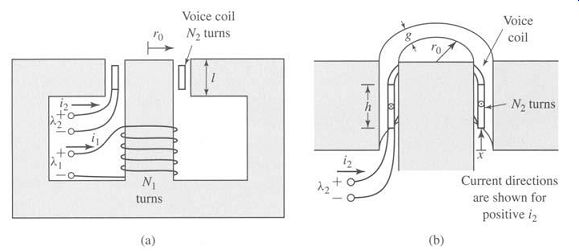
FIG. 37 Loudspeaker for Problem 25.

b. Calculate the self-inductance of each coil.

c. Calculate the mutual inductance between the coils. (Hint: Assume that current is applied to the voice coil, and calculate the flux linkages of coil 1. Note that these flux linkages vary with the displacement x.)

d. Calculate the force on the voice coil from the coenergy W~a.

26. Repeat Example 8 with the samarium-cobalt magnet replaced by a neodymium-iron-boron magnet.

27. The magnetic structure of FIG. 38 is a schematic view of a system designed to support a block of magnetic material (/x --+ c~) of mass M against the force of gravity. The system includes a permanent magnet and a winding. Under normal conditions, the force is supplied by the permanent magnet alone. The function of the winding is to counteract the field produced by the magnet so that the mass can be removed from the device. The system is designed such that the air gaps at each side of the mass remain constant at length go~2.

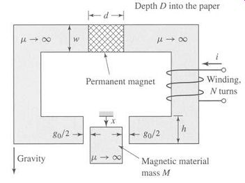
FIG. 38 Magnetic support system for Problem 27.

Assume that the permanent magnet can be represented by a linear characteristic of the form

Bm =/ZR(HmHc)

and that the winding direction is such that positive winding current reduces the air-gap flux produced by the permanent magnet. Neglect the effects of magnetic fringing.

a. Assume the winding current to be zero. (i) Find the force fnd acting on the mass in the x direction due to the permanent magnet alone as a function of x (0 < x < h). (ii) Find the maximum mass Mmax that can be supported against gravity for 0 < x < h.

b. For M = Mmax/2, find the minimum current required to ensure that the mass will fall out of the system when the current is applied.

28. Winding 1 in the loudspeaker of Problem 25 (FIG. 37) is replaced by a permanent magnet as shown in FIG. 39. The magnet can be represented by the linear characteristic Bm -/ZR (Hm -Hc).

a. Assuming the voice coil current to be zero, (i2 = 0), calculate the magnetic flux density in the air gap.

b. Calculate the flux linkage of the voice coil due to the permanent magnet as a function of the displacement x.

c. Calculate the coenergy W~d(i2, x) assuming that the voice coil current is sufficiently small so that the component of W~d due to the voice coil self inductance can be ignored.

d. Calculate the force on the voice coil.

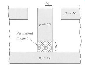
FIG. 39 Central core of loudspeaker of FIG. 37 with winding 1 replaced by a permanent magnet (Problem 28).

29. FIG. 40 shows a circularly symmetric system in which a moveable plunger (constrained to move only in the vertical direction) is supported by a spring of spring constant K = 5.28 N/m. The system is excited by a samarium-cobalt permanent-magnet in the shape of a washer of outer radius R3, inner radius R2, and thickness tm. The system dimensions are: R1 -2.1 cm, R2 = 4 cm, R3 = 4.5 cm h -1 cm, g = 1 mm, tm --= 3 mm

The equilibrium position of the plunger is observed to be x 1.0 mm.

a. Find the magnetic flux density Bg in the fixed gap and Bx in the variable gap.

b. Calculate the x-directed magnetic force pulling down on the plunger.

c. The spring force is of the form f_spring -K (X0 x). Find X0.

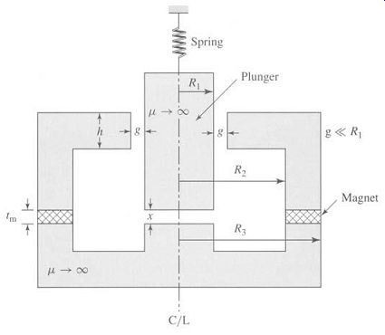
FIG. 40 Permanent-magnet system for Problem 29.

30. The plunger of a solenoid is connected to a spring. The spring force is given by f = K0(0.9a x), where x is the air-gap length. The inductance of the solenoid is of the form L = Lo(1 x/a), and its winding resistance is R. The plunger is initially stationary at position x = 0.9a when a dc voltage of magnitude V0 is applied to the solenoid.

a. Find an expression for the force as a function of time required to hold the plunger at position a/2.

b. If the plunger is then released and allowed to come to equilibrium, find the equilibrium position X0. You may assume that this position falls in the range 0 _< X0 < a.

31. Consider the solenoid system of Problem 30.

Assume the following parameter values:

L0=4.0mH a--2.2cm

R=1.5~ K0=3.5N/cm

The plunger has mass M = 0.2 kg.

Assume the coil to be connected to a dc source of magnitude 4 A. Neglect any effects of gravity.

a. Find the equilibrium displacement X0.

b. Write the dynamic equations of motion for the system.

c. Linearize these dynamic equations for incremental motion of the system around its equilibrium position.

d. If the plunger is displaced by an incremental distance E from its equilibrium position X0 and released with zero velocity at time t = 0, find (i) The resultant motion of the plunger as a function of time, and (ii) The corresponding time-varying component of current induced across the coil terminals.

32. The solenoid of Problem 31 is now connected to a dc voltage source of magnitude 6 V.

a. Find the equilibrium displacement X0.

b. Write the dynamic equations of motion for the system.

c. Linearize these dynamic equations for incremental motion of the system around its equilibrium position.

33. Consider the single-coil rotor of Example 1. Assume the rotor winding to be carrying a constant current of 18 A and the rotor to have a moment of inertia J = 0.0125 kg. m^2.

a. Find the equilibrium position of the rotor. Is it stable?

b. Write the dynamic equations for the system.

c. Find the natural frequency in hertz for incremental rotor motion around this equilibrium position.

34. Consider a solenoid magnet similar to that of Example 10 (FIG. 24) except that the length of the cylindrical plunger is reduced to a + h. Derive the dynamic equations of motion of the system.