Electric Machinery--Transformers

Before we proceed with a study of electric machinery, it is desirable to discuss certain aspects of the theory of magnetically-coupled circuits, with emphasis on transformer action. Although the static transformer is not an energy conversion device, it is an indispensable component in many energy conversion systems.

A significant component of ac power systems, it makes possible electric generation at the most economical generator voltage, power transfer at the most economical transmission voltage, and power utilization at the most suitable voltage for the particular utilization device. The transformer is also widely used in low-power, low-current electronic and control circuits for performing such functions as matching the impedances of a source and its load for maximum power transfer, isolating one circuit from another, or isolating direct current while maintaining ac continuity between two circuits.

The transformer is one of the simpler devices comprising two or more electric circuits coupled by a common magnetic circuit. Its analysis involves many of the principles essential to the study of electric machinery. Thus, our study of the transformer will serve as a bridge between the introduction to magnetic-circuit analysis of Section 1 and the more detailed study of electric machinery to follow.

1. INTRODUCTION TO TRANSFORMERS

Essentially, a transformer consists of two or more windings coupled by mutual magnetic flux. If one of these windings, the primary, is connected to an alternating-voltage source, an alternating flux will be produced whose amplitude will depend on the primary voltage, the frequency of the applied voltage, and the number of turns. The mutual flux will link the other winding, the secondary, 1 and will induce a voltage in it whose value will depend on the number of secondary turns as well as the magnitude of the mutual flux and the frequency. By properly proportioning the number of primary and secondary turns, almost any desired voltage ratio, or ratio of transformation, can be obtained.

[1. It is conventional to think of the "input" to the transformer as the primary and the "output" as the secondary. However, in many applications, power can flow either way and the concept of primary and secondary windings can become confusing. An alternate terminology, which refers to the windings as "high-voltage" and "low-voltage," is often used and eliminates this confusion. ]

The essence of transformer action requires only the existence of time-varying mutual flux linking two windings. Such action can occur for two windings coupled through air, but coupling between the windings can be made much more effectively using a core of iron or other ferromagnetic material, because most of the flux is then confined to a definite, high-permeability path linking the windings. Such a transformer is commonly called an iron-core transformer. Most transformers are of this type. The following discussion is concerned almost wholly with iron-core transformers.

As discussed in Section 4, to reduce the losses caused by eddy currents in the core, the magnetic circuit usually consists of a stack of thin laminations. Two common types of construction are shown schematically in Fig. 1. In the core type (Fig. 1 a)

the windings are wound around two legs of a rectangular magnetic core; in the shell type (Fig. lb) the windings are wound around the center leg of a three-legged core.

Silicon-steel laminations 0.014 in thick are generally used for transformers operating at frequencies below a few hundred hertz. Silicon steel has the desirable properties of low cost, low core loss, and high permeability at high flux densities (1.0 to 1.5 T). The cores of small transformers used in communication circuits at high frequencies and low energy levels are sometimes made of compressed powdered ferromagnetic alloys known as ferrites.

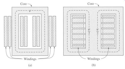
FIG. 1 Schematic views of (a) core-type and (b) shell-type transformers.

In each of these configurations, most of the flux is confined to the core and therefore links both windings. The windings also produce additional flux, known as leakage flux, which links one winding without linking the other. Although leakage flux is a small fraction of the total flux, it plays an important role in determining the behavior of the transformer. In practical transformers, leakage is reduced by subdividing the windings into sections placed as close together as possible. In the core-type construction, each winding consists of two sections, one section on each of the two legs of the core, the primary and secondary windings being concentric coils.

In the shell-type construction, variations of the concentric-winding arrangement may be used, or the windings may consist of a number of thin "pancake" coils assembled in a stack with primary and secondary coils interleaved.

FIG. 2 illustrates the internal construction of a distribution transformer such as is used in public utility systems to provide the appropriate voltage for use by residential consumers. A large power transformer is shown in Fig. 3.

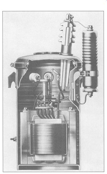
FIG. 2 Cutaway view of self-protected distribution transformer typical of sizes 2 to 25 kVA, 7200:240/120 V. Only one high-voltage insulator and lightning arrester is needed because one side of the 7200-V line and one side of the primary are grounded.

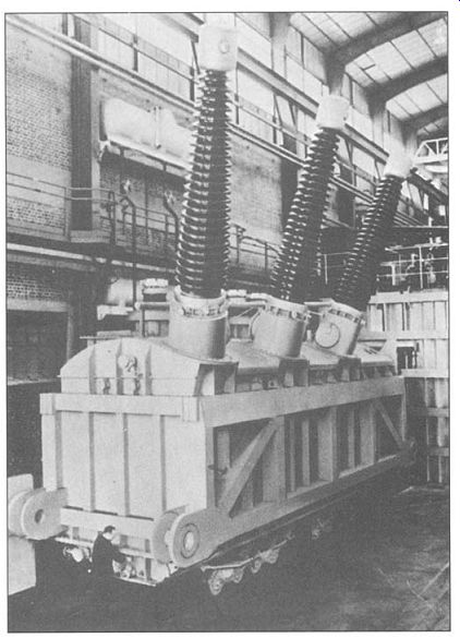
FIG. 3 A 660-MVA three-phase 50-Hz transformer used to step up generator voltage of 20 kV to transmission voltage of 405 kV.

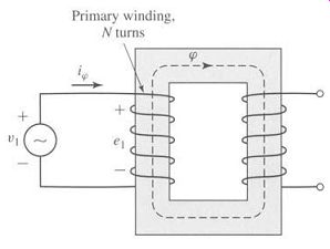
FIG. 4 Transformer with open secondary.

2. NO-LOAD CONDITIONS

FIG. 4 shows in schematic form a transformer with its secondary circuit open and an alternating voltage vl applied to its primary terminals. To simplify the drawings, it is common on schematic diagrams of transformers to show the primary and secondary windings as if they were on separate legs of the core, as in Fig. 4, even though the windings are actually interleaved in practice. As discussed in Section 4, a small steady-state current i~, called the exciting current, flows in the primary and establishes an alternating flux in the magnetic circuit. 2 This flux induces an emf in the primary equal to

(EQN. 1)

~.1 -flux linkage of the primary winding

~0 = flux in the core linking both windings

N1 -number of turns in the primary winding

The voltage el is in volts when q9 is in webers. This emf, together with the voltage drop in the primary resistance R1, must balance the applied voltage

(EQN. 2)

Note that for the purposes of the current discussion, we are neglecting the effects of primary leakage flux, which will add an additional induced-emf term in Eq. 2. In typical transformers, this flux is a small percentage of the core flux, and it is quite justifiable to neglect it for our current purposes. It does however play an important role in the behavior of transformers and is discussed in some detail in Section 4.

In most large transformers, the no-load resistance drop is very small indeed, and the induced emf el very nearly equals the applied voltage V1. Furthermore, the waveforms of voltage and flux are very nearly sinusoidal. The analysis can then be greatly simplified, as we have shown in Section 4. Thus, if the instantaneous flux is

(EQN. 3)

the induced voltage is

(EQN. 4)

where q~max is the maximum value of the flux and co = 2:r f, the frequency being f Hz. For the current and voltage reference directions shown in Fig. 4, the induced emf leads the flux by 90 °. The rms value of the induced emf el is

(EQN. 5)

If the resistive voltage drop is negligible, the counter emf equals the applied voltage. Under these conditions, if a sinusoidal voltage is applied to a winding, a sinusoidally varying core flux must be established whose maximum value CP max satisfies the requirement that E1 in Eq. 5 equal the rms value V1 of the applied voltage; thus:

(EQN. 6)

[In general, the exciting current corresponds to the net ampere-turns (mmf) acting on the magnetic circuit, and it is not possible to distinguish whether it flows in the primary or secondary winding or partially in each winding. ]

Under these conditions, the core flux is determined solely by the applied voltage, its frequency, and the number of turns in the winding. This important relation applies not only to transformers but also to any device operated with a sinusoidally-alternating impressed voltage, as long as the resistance and leakage-inductance voltage drops are negligible. The core flux is fixed by the applied voltage, and the required exciting current is determined by the magnetic properties of the core; the exciting current must adjust itself so as to produce the mmf required to create the flux demanded by Eq. 6.

Because of the nonlinear magnetic properties of iron, the waveform of the exciting current differs from the waveform of the flux. A curve of the exciting current as a function of time can be found graphically from the ac hysteresis loop, as is discussed in Section 4 and shown in Fig. 1.11.

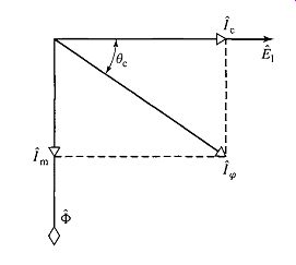
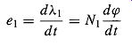
FIG. 5 No-load phasor diagram.

If the exciting current is analyzed by Fourier-series methods, it is found to consist of a fundamental component and a series of odd harmonics. The fundamental component can, in turn, be resolved into two components, one in phase with the counter emf and the other lagging the counter emf by 90 °. The in-phase component supplies the power absorbed by hysteresis and eddy-current losses in the core. It is referred to as core-loss component of the exciting current. When the core-loss component is subtracted from the total exciting current, the remainder is called the magnetizing current. It comprises a fundamental component lagging the counter emf by 90 °, together with all the harmonics. The principal harmonic is the third. For typical power transformers, the third harmonic usually is about 40 percent of the exciting current.

Except in problems concerned directly with the effects of harmonic currents, the peculiarities of the exciting-current waveform usually need not be taken into account, because the exciting current itself is small, especially in large transformers.

For example, the exciting current of a typical power transformer is about 1 to 2 percent of full-load current. Consequently the effects of the harmonics usually are swamped out by the sinusoidal-currents supplied to other linear elements in the circuit. The exciting current can then be represented by an equivalent sinusoidal current which has the same rms value and frequency and produces the same average power as the actual exciting current. Such representation is essential to the construction of a phasor diagram, which represents the phase relationship between the various voltages and currents in a system in vector form. Each signal is represented by a phasor whose length is proportional to the amplitude of the signal and whose angle is equal to the phase angle of that signal as measured with respect to a chosen reference signal.

In Fig. 5, the phasors/~1 and + respectively, represent the rms values of the induced emf and the flux. The phasor i~ represents the rms value of the equivalent sinusoidal exciting current. It lags the induced emf/~1 by a phase angle 0c.

The core loss Pc, equal to the product of the in-phase components of the/~1 and i¢, is given by:

(EQN. 7)

The component ic in phase with /~1 is the core-loss current. The component Im in phase with the flux represents an equivalent sine wave current having the same rms value as the magnetizing current. Typical exciting volt-ampere and core-loss characteristics of high-quality silicon steel used for power and distribution transformer laminations are shown in Figs. 1.12 and 1.14.

3. EFFECT OF SECONDARY CURRENT; IDEAL TRANSFORMER

As a first approximation to a quantitative theory, consider a transformer with a primary winding of N1 turns and a secondary winding of N2 turns, as shown schematically in Fig. 6. Notice that the secondary current is defined as positive out of the winding; thus positive secondary current produces an mmf in the opposite direction from that created by positive primary current. Let the properties of this transformer be idealized under the assumption that winding resistances are negligible, that all the flux is confined to the core and links both windings (i.e., leakage flux is assumed negligible), that there are no losses in the core, and that the permeability of the core is so high that only a negligible exciting mmf is required to establish the flux. These properties are closely approached but never actually attained in practical transformers. A hypothetical transformer having these properties is often called an ideal transformer.

Under the above assumptions, when a time-varying voltage V1 is impressed on the primary terminals, a core flux q9 must be established such that the counter emf el equals the impressed voltage. Thus

(EQN. 8)

The core flux also links the secondary and produces an induced emf e2, and an equal secondary terminal voltage re, given by

(EQN. 9)

FIG. 6 Ideal transformer and load.

From the ratio of Eqs. 8 and 9

(EQN. 10)

Thus an ideal transformer transforms voltages in the direct ratio of the turns in its windings.

Now let a load be connected to the secondary. A current i2 and an mmf N2i2 are then present in the secondary. Since the core permeability is assumed very large and since the impressed primary voltage sets the core flux as specified by Eq. 8, the core flux is unchanged by the presence of a load on the secondary, and hence the net exciting mmf acting on the core will not change and hence will remain negligible. Thus:

(EQN. 11)

From Eq. 11 we see that a compensating primary mmf must result to cancel that of the secondary. Hence:

(EQN. 12)

Thus we see that the requirement that the net mmf remain unchanged is the means by which the primary "knows" of the presence of load current in the secondary; any change in mmf flowing in the secondary as the result of a load must be accompanied by a corresponding change in the primary mmf. Note that for the reference directions shown in Fig. 6 the mmf's of i1 and i2 are in opposite directions and therefore compensate. The net mmf acting on the core therefore is zero, in accordance with the assumption that the exciting current of an ideal transformer is zero.

From Eq. 12 -(EQN. 13)

Thus an ideal transformer transforms currents in the inverse ratio of the turns in its windings.

Also notice from Eqs. 10 and 13 that

(EQN. 14)

... i.e., instantaneous power input to the primary equals the instantaneous power output from the secondary, a necessary condition because all dissipative and energy storage mechanisms in the transformer have been neglected.

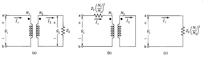
FIG. 7 Three circuits which are identical at terminals ab when the transformer is ideal.

An additional property of the ideal transformer can be seen by considering the case of a sinusoidal applied voltage and an impedance load. Phasor symbolism can be used. The circuit is shown in simplified form in Fig. 7a, in which the dot-marked terminals of the transformer correspond to the similarly marked terminals in Fig. 6. The dot markings indicate terminals of corresponding polarity; i.e., if one follows through the primary and secondary windings of Fig. 6, beginning at their dot-marked terminals, one will find that both windings encircle the core in the same direction with respect to the flux. Therefore, if one compares the voltages of the two windings, the voltages from a dot-marked to an unmarked terminal will be of the same instantaneous polarity for primary and secondary. In other words, the voltages fZl and f'2 in Fig. 7a are in phase. Also currents i1 and i2 are in phase as seen from Eq. 12. Note again that the polarity of i1 is defined as into the dotted terminal and the polarity of i2 is defined as out of the dotted terminal.

We next investigate the impendence transformation properties of the ideal transformer. In phasor form, Eqs. 10 and 13 can be expressed as

(EQN. 15)

(EQN. 16)

(EQN. 17)

Noting that the load impedance Z2 is related to the secondary voltages and currents

(EQN. 18)

where Z2 is the complex impedance of the load. Consequently, as far as its effect is concerned, an impedance Z2 in the secondary circuit can be replaced by an equivalent impedance Z1 in the primary circuit, provided that

(EQN. 19)

Thus, the three circuits of Fig. 7 are indistinguishable as far as their performance viewed from terminals ab is concerned. Transferring an impedance from one side of a transformer to the other in this fashion is called referring the impedance to the

other side; impedances transform as the square of the turns ratio. In a similar manner, voltages and currents can be referred to one side or the other by using Eqs. 15 and 16 to evaluate the equivalent voltage and current on that side.

To summarize, in an ideal transformer, voltages are transformed in the direct ratio of turns, currents in the inverse ratio, and impedances in the direct ratio squared; power and voltamperes are unchanged.

4. TRANSFORMER REACTANCES AND EQUIVALENT CIRCUITS

The departures of an actual transformer from those of an ideal transformer must be included to a greater or lesser degree in most analyses of transformer performance.

A more complete model must take into account the effects of winding resistances, leakage fluxes, and finite exciting current due to the finite (and indeed nonlinear) permeability of the core. In some cases, the capacitances of the windings also have important effects, notably in problems involving transformer behavior at frequencies above the audio range or during rapidly changing transient conditions such as those encountered in power system transformers as a result of voltage surges caused by lightning or switching transients. The analysis of these high-frequency problems is beyond the scope of the present treatment however, and accordingly the capacitances of the windings will be neglected.

Two methods of analysis by which departures from the ideal can be taken into account are (1) an equivalent-circuit technique based on physical reasoning and (2) a mathematical approach based on the classical theory of magnetically coupled circuits.

Both methods are in everyday use, and both have very close parallels in the theories of rotating machines. Because it offers an excellent example of the thought process involved in translating physical concepts to a quantitative theory, the equivalent circuit technique is presented here.

To begin the development of a transformer equivalent circuit, we first consider the primary winding. The total flux linking the primary winding can be divided into two components: the resultant mutual flux, confined essentially to the iron core and produced by the combined effect of the primary and secondary currents, and the primary leakage flux, which links only the primary. These components are identified in the schematic transformer shown in Fig. 9, where for simplicity the primary and secondary windings are shown on opposite legs of the core. In an actual transformer with interleaved windings, the details of the flux distribution are more complicated, but the essential features remain the same.

FIG. 9 Schematic view of mutual and leakage fluxes in a transformer.

The leakage flux induces voltage in the primary winding which adds to that produced by the mutual flux. Because the leakage path is largely in air, this flux and the voltage induced by it vary linearly with primary current i l. It can therefore be represented by a primary leakage inductance Lll (equal to the leakage-flux linkages with the primary per unit of primary current). The corresponding primary leakage reactance Xll is found as

(EQN. 20)

In addition, there will be a voltage drop in the primary resistance R1.

We now see that the primary terminal voltage (11 consists of three components: the il R1 drop in the primary resistance, the i l Xll drop arising from primary leakage flux, and the emf/~1 induced in the primary by the resultant mutual flux. Fig. 10a shows an equivalent circuit for the primary winding which includes each of these voltages.

[In fact, the exciting current corresponds to the net mmf acting on the transformer core and cannot, in general, be considered to flow in the primary alone. However, for the purposes of this discussion, this distinction is not significant. ]

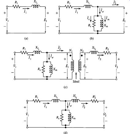
FIG. 10 Steps in the development of the transformer equivalent circuit.

The resultant mutual flux links both the primary and secondary windings and is created by their combined mmf's. It is convenient to treat these mmf's by considering that the primary current must meet two requirements of the magnetic circuit: It must not only produce the mmf required to produce the resultant mutual flux, but it must also counteract the effect of the secondary mmf which acts to demagnetize the core.

An alternative viewpoint is that the primary current must not only magnetize the core, it must also supply current to the load connected to the secondary. According to this picture, it is convenient to resolve the primary current into two components: an exciting component and a load component. The exciting component i~ is defined as the additional primary current required to produce the resultant mutual flux. It is a nonsinusoidal current of the nature described in Section 2.2. 3 The load component i' 2 is defined as the component current in the primary which would exactly counteract the mmf of secondary current i2.

Since it is the exciting component which produces the core flux, the net mmf must equal N1 i~0 and thus we see that:

(EQN. 21)

(EQN. 22)

From Eq. 22, we see that the load component of the primary current equals the secondary current referred to the primary as in an ideal transformer.

The exciting current can be treated as an equivalent sinusoidal current i~0, in the manner described in Section 2, and can be resolved into a core-loss component ic in phase with the emf E1 and a magnetizing component lm lagging E1 by 90 °. In the equivalent circuit (Fig. 10b) the equivalent sinusoidal exciting current is accounted for by means of a shunt branch connected across El, comprising a coreloss resistance Rc in parallel with a magnetizing inductance Lm whose reactance, known as the magnetizing reactance, is given by

(EQN. 23)

In the equivalent circuit of (Fig. 10b) the power E 2/Rc accounts for the core loss due to the resultant mutual flux. Rc is referred to as the magnetizing resistance or core-loss resistance and together with Xm forms the excitation branch of the equivalent circuit, and we will refer to the parallel combination of Rc and Xm as the exciting impedance Z~. When Rc is assumed constant, the core loss is thereby assumed to vary as E 2 or (for sine waves) as ~2ax f2, where ~bmax is the maximum value of the resultant mutual flux. Strictly speaking, the magnetizing reactance Xm varies with the saturation of the iron. When Xm is assumed constant, the magnetizing current is thereby assumed to be independent of frequency and directly proportional to the resultant mutual flux. Both Rc and Xm are usually determined at rated voltage and frequency; they are then assumed to remain constant for the small departures from rated values associated with normal operation.

We will next add to our equivalent circuit a representation of the secondary winding. We begin by recognizing that the resultant mutual flux + induces an emf/~2 in the secondary, and since this flux links both windings, the induced-emf ratio must equal the winding turns ratio, i.e.,

(EQN. 24)

... just as in an ideal transformer. This voltage transformation and the current transformation of Eq. 22 can be accounted for by introducing an ideal transformer in the equivalent circuit, as in Fig. 10c. Just as is the case for the primary winding, the emf E2 is not the secondary terminal voltage, however, because of the secondary resistance R2 and because the secondary current i2 creates secondary leakage flux (see Fig. 9). The secondary terminal voltage 92 differs from the induced voltage/~2 by the voltage drops due to secondary resistance R2 and secondary leakage reactance Xl: (corresponding to the secondary leakage inductance L12), as in the portion of the complete transformer equivalent circuit (Fig. 10c) to the fight of/~2.

From the equivalent circuit of Fig. 10, the actual transformer therefore can be seen to be equivalent to an ideal transformer plus external impedances. By referring all quantities to the primary or secondary, the ideal transformer in Fig. 10c can be moved out to the fight or left, respectively, of the equivalent circuit. This is almost invariably done, and the equivalent circuit is usually drawn as in Fig. 10d, with the ideal transformer not shown and all voltages, currents, and impedances referred to either the primary or secondary winding. Specifically, for Fig. 10d,

(EQN. 25)

(EQN. 26)

(EQN. 27)

The circuit of Fig. 10d is called the equivalent-T circuit for a transformer.

In Fig. 10d, in which the secondary quantities are referred to the primary, the referred secondary values are indicated with primes, for example, X' and R~, to distinguish them from the actual values of Fig. 10c. In the discussion that follows we almost always deal with referred values, and the primes will be omitted. One must simply keep in mind the side of the transformers to which all quantities have been referred.

5. ENGINEERING ASPECTS OF TRANSFORMER ANALYSIS

In engineering analyses involving the transformer as a circuit element, it is customary to adopt one of several approximate forms of the equivalent circuit of Fig. 10 rather than the full circuit. The approximations chosen in a particular case depend largely on physical reasoning based on orders of magnitude of the neglected quantities. The more common approximations are presented in this section. In addition, test methods are given for determining the transformer constants.

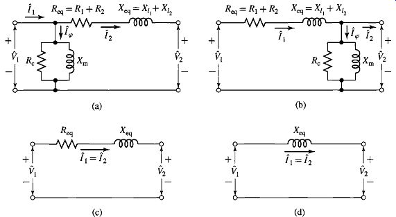
FIG. 12 Approximate transformer equivalent circuits.

The approximate equivalent circuits commonly used for constant-frequency power transformer analyses are summarized for comparison in Fig. 12. All quantities in these circuits are referred to either the primary or the secondary, and the ideal transformer is not shown.

Computations can often be greatly simplified by moving the shunt branch representing the exciting current out from the middle of the T circuit to either the primary or the secondary terminals, as in Fig. 12a and b. These forms of the equivalent circuit are referred to as cantilever circuits. The series branch is the combined resistance and leakage reactance of the primary and secondary, referred to the same side. This impedance is sometimes called the equivalent series impedance and its components the equivalent series resistance Req and equivalent series reactance Xeq, as shown in Fig. 12a and b.

As compared to the equivalent-T circuit of Fig. 10d, the cantilever circuit is in error in that it neglects the voltage drop in the primary or secondary leakage impedance caused by the exciting current. Because the impedance of the exciting branch is typically quite large in large power transformers, the corresponding exciting current is quite small. This error is insignificant in most situations involving large transformers.

Further analytical simplification results from neglecting the exciting current entirely, as in Fig. 12c, in which the transformer is represented as an equivalent series impedance. If the transformer is large (several hundred kilo-voltamperes or more), the equivalent resistance Req is small compared with the equivalent reactance Xeq and can frequently be neglected, giving the equivalent circuit of Fig. 12d. The circuits of Fig. 12c and d are sufficiently accurate for most ordinary power system problems and are used in all but the most detailed analyses. Finally, in situations where the currents and voltages are determined almost wholly by the circuits external to the transformer or when a high degree of accuracy is not required, the entire transformer impedance can be neglected and the transformer considered to be ideal, as in Section 2.3.

The circuits of Fig. 12 have the additional advantage that the total equivalent resistance Req and equivalent reactance Xeq can be found from a very simple test in which one terminal is short-circuited. On the other hand, the process of determination of the individual leakage reactances X11 and X12 and a complete set of parameters for the equivalent-T circuit of Fig. 10c is more difficult. Example 4 illustrates that due to the voltage drop across leakage impedances, the ratio of the measured voltages of a transformer will not be identically equal to the idealized voltage ratio which would be measured if the transformer were ideal. In fact, without some apriori knowledge of the turns ratio (based for example upon knowledge of the internal construction of the transformer), it is not possible to make a set of measurements which uniquely determine the turns ratio, the magnetizing inductance, and the individual leakage impedances.

It can be shown that, simply from terminal measurements, neither the turns ratio, the magnetizing reactance, or the leakage reactances are unique characteristics of a transformer equivalent circuit. For example, the turns ratio can be chosen arbitrarily and for each choice of turns ratio, there will be a corresponding set of values for the leakage and magnetizing reactances which matches the measured characteristic.

Each of the resultant equivalent circuits will have the same electrical terminal characteristics, a fact which has the fortunate consequence that any self-consistent set of empirically determined parameters will adequately represent the transformer.

Two very simple tests serve to determine the parameters of the equivalent circuits of Fig. 10 and 2.12. These consist of measuring the input voltage, current, and power to the primary, first with the secondary short-circuited and then with the secondary open-circuited.

Short-Circuit Test The short-circuit test can be used to find the equivalent series impedance Req -kj Xeq. Although the choice of winding to short-circuit is arbitrary, for the sake of this discussion we will consider the short circuit to be applied to the transformer secondary and voltage applied to primary. For convenience, the high-voltage side is usually taken as the primary in this test. Because the equivalent series impedance in a typical transformer is relatively small, typically an applied primary voltage on the order of 10 to 15 percent or less of the rated value will result in rated current.

FIG. 15a shows the equivalent circuit with transformer secondary impedance referred to the primary side and a short circuit applied to the secondary. The shortcircuit impedance Zsc looking into the primary under these conditions is ...

(EQN. 28)

Because the impedance Z~ of the exciting branch is much larger than that of the secondary leakage impedance (which will be true unless the core is heavily saturated by excessive voltage applied to the primary; certainly not the case here), the shortcircuit impedance can be approximated as

(EQN. 29)

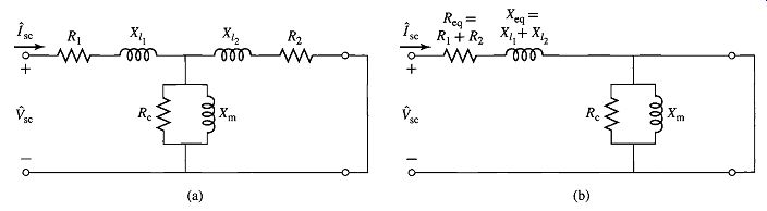
FIG. 15 Equivalent circuit with short-circuited secondary. (a) Complete equivalent circuit. (b) Cantilever equivalent circuit with the exciting branch at the transformer secondary.

Note that the approximation made here is equivalent to the approximation made in reducing the equivalent-T circuit to the cantilever equivalent. This can be seen from Fig. 15b; the impedance seen at the input of this equivalent circuit is clearly Zsc = Zeq -Req qj Xeq since the exciting branch is directly shorted out by the short on the secondary.

Typically the instrumentation used for this test will measure the rms magnitude of the applied voltage Vsc, the short-circuit current Isc, and the power Psc. Based upon these three measurements, the equivalent resistance and reactance (referred to the primary) can be found from...

(EQN. 30)

(EQN. 31)

(EQN. 32)

... where the symbol II indicates the magnitude of the enclosed complex quantity.

The equivalent impedance can, of course, be referred from one side to the other in the usual manner. On the rare occasions when the equivalent-T circuit in Fig. 10d must be resorted to, approximate values of the individual primary and secondary resistances and leakage reactances can be obtained by assuming that R1 = R2 - 0.5 Req and X1, = X12 = 0.5Xeq when all impedances are referred to the same side.

Strictly speaking, of course, it is possible to measure R l and R2 directly by a dc resistance measurement on each winding (and then referring one or the other to the other side of the idea transformer). However, as has been discussed, no such simple test exists for the leakage reactances X1, and X12.

Open-Circuit Test

The open-circuit test is performed with the secondary open-circuited and rated voltage impressed on the primary. Under this condition an exciting current of a few percent of full-load current (less on large transformers and more on smaller ones) is obtained. Rated voltage is chosen to insure that the magnetizing reactance will be operating at a flux level close to that which will exist under normal operating conditions. If the transformer is to be used at other than its rated voltage, the test should be done at that voltage. For convenience, the low-voltage side is usually taken as the primary in this test. If the primary in this test is chosen to be the opposite winding from that of the short-circuit test, one must of course be careful to refer the various measured impedances to the same side of the transformer in order to obtain a self-consistent set of parameter values.

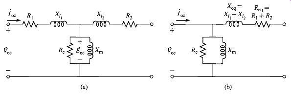
FIG. 16 Equivalent circuit with open-circuited secondary. (a) Complete equivalent circuit. (b) Cantilever equivalent circuit with the exciting branch at the transformer primary.

FIG. 16a shows the equivalent circuit with the transformer secondary impedance referred to the primary side and the secondary open-circuited. The open-circuit impedance Zoc looking into the primary under these conditions is

(EQN. 33)

Because the impedance of the exciting branch is quite large, the voltage drop in the primary leakage impedance caused by the exciting current is typically negligible, and the primary impressed voltage f'oc very nearly equals the emf/~oc induced by the resultant core flux. Similarly, the primary I2cR1 loss caused by the exciting current is negligible, so that the power input Poc very nearly equals the core loss 2 Eoc/Re. As a result, it is common to ignore the primary leakage impedance and to approximate the open-circuit impedance as being equal to the magnetizing impedance

(EQN. 34)

Note that the approximation made here is equivalent to the approximation made in reducing the equivalent-T circuit to the cantilever equivalent circuit of Fig. 16b; the impedance seen at the input of this equivalent circuit is clearly Z~0 since no current will flow in the open-circuited secondary.

As with the short-circuit test, typically the instrumentation used for this test will measure the rms magnitude of the applied voltage, Voc, the open-circuit current Ioc and the power Poc. Neglecting the primarily leakage impedance and based upon these three measurements, the magnetizing resistance and reactance (referred to the primary) can be found from

(EQN. 36)

(EQN. 37)

The values obtained are, of course, referred to the side used as the primary in this test.

The open-circuit test can be used to obtain the core loss for efficiency computations and to check the magnitude of the exciting current. Sometimes the voltage at the terminals of the open-circuited secondary is measured as a check on the turns ratio.

Note that, if desired, a slightly more accurate calculation of Xm and Rc by retaining the measurements of R1 and Xll obtained from the short-circuit test (referred to the proper side of the transformer) and basing the derivation on Eq. 33. However, such additional effort is rarely necessary for the purposes of engineering accuracy.

6. AUTOTRANSFORMERS; MULTI-WINDING TRANSFORMERS

The principles discussed in previous sections have been developed with specific reference to two-winding transformers. They are also applicable to transformers with other winding configurations. Aspects relating to autotransformers and multi-winding transformers are considered in this section.

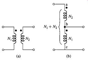
FIG. 17 (a) Two-winding transformer. (b) Connection as an autotransformer.

6.1 Autotransformers

In Fig. 17a, a two-winding transformer is shown with N1 and N2 turns on the primary and secondary windings respectively. Substantially the same transformation effect on voltages, currents, and impedances can be obtained when these windings are connected as shown in Fig. 17b. Note that, however, in Fig. 17b, winding bc is common to both the primary and secondary circuits. This type of transformer is called an autotransformer. It is little more than a normal transformer connected in a special way.

One important difference between the two-winding transformer and the autotransformer is that the windings of the two-winding transformer are electrically isolated whereas those of the autotransformer are connected directly together. Also, in the autotransformer connection, winding ab must be provided with extra insulation since it must be insulated against the full maximum voltage of the autotransformer.

Autotransformers have lower leakage reactances, lower losses, and smaller exciting current and cost less than two-winding transformers when the voltage ratio does not differ too greatly from 1:1.

The following example illustrates the benefits of an autotransformer for those situations where electrical isolation between the primary and secondary windings is not an important consideration.

6.2 Multiwinding Transformers

Transformers having three or more windings, known as multiwinding or multicircuit transformers, are often used to interconnect three or more circuits which may have different voltages. For these purposes a multiwinding transformer costs less and is more efficient than an equivalent number of two-winding transformers. Transformers having a primary and multiple secondaries are frequently found in multiple-output dc power supplies for electronic applications. Distribution transformers used to supply power for domestic purposes usually have two 120-V secondaries connected in series.

Circuits for lighting and low-power applications are connected across each of the 120-V windings, while electric ranges, domestic hot-water heaters, clothes-dryers, and other high-power loads are supplied with 240-V power from the series-connected secondaries.

Similarly, a large distribution system may be supplied through a three-phase bank of multiwinding transformers from two or more transmission systems having different voltages. In addition, the three-phase transformer banks used to interconnect two transmission systems of different voltages often have a third, or tertiary, set of windings to provide voltage for auxiliary power purposes in substations or to supply a local distribution system. Static capacitors or synchronous condensers may be connected to the tertiary windings for power factor correction or voltage regulation.

Sometimes A-connected tertiary windings are put on three-phase banks to provide a low-impedance path for third harmonic components of the exciting current to reduce third-harmonic components of the neutral voltage.

Some of the issues arising in the use of multiwinding transformers are associated with the effects of leakage impedances on voltage regulation, short-circuit currents, and division of load among circuits. These problems can be solved by an equivalent-circuit technique similar to that used in dealing with two-circuit transformers.

The equivalent circuits of multiwinding transformers are more complicated than in the two-winding case because they must take into account the leakage impedances associated with each pair of windings. Typically, in these equivalent circuits, all quantities are referred to a common base, either by use of the appropriate turns ratios as referring factors or by expressing all quantities in per unit. The exciting current usually is neglected.

7. TRANSFORMERS IN THREE-PHASE CIRCUITS

Three single-phase transformers can be connected to form a three-phase transformer bank in any of the four ways shown in Fig. 19. In all four parts of this figure, the windings at the left are the primaries, those at the right are the secondaries, and any primary winding in one transformer corresponds to the secondary winding drawn parallel to it.

Also shown are the voltages and currents resulting from balanced impressed primary line-to-line voltages V and line currents I when the ratio of primary-to-secondary turns N1/N2 = a and ideal transformers are assumed. 4 Note that the rated voltages and currents at the primary and secondary of the three-phase transformer bank depends upon the connection used but that the rated kVA of the three-phase bank is three times that of the individual single-phase transformers, regardless of the connection.

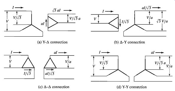
FIG. 19 Common three-phase transformer connections; the transformer windings are indicated by the heavy lines.

The Y-A connection is commonly used in stepping down from a high voltage to a medium or low voltage. One reason is that a neutral is thereby provided for grounding on the high-voltage side, a procedure which can be shown to be desirable in many cases. Conversely, the A-Y connection is commonly used for stepping up to a high voltage. The A-A connection has the advantage that one transformer can be removed for repair or maintenance while the remaining two continue to function as a three-phase bank with the rating reduced to 58 percent of that of the original bank; this is known as the open-delta, or V, connection. The Y-Y connection is seldom used because of difficulties with exciting-current phenomena.

[ Because there is no neutral connection to carry harmonics of the exciting current, harmonic voltages are produced which significantly distort the transformer voltages. ]

Instead of three single-phase transformers, a three-phase bank may consist of one three-phase transformer having all six windings on a common multi-legged core and contained in a single tank. Advantages of three-phase transformers over connections of three single-phase transformers are that they cost less, weigh less, require less floor space, and have somewhat higher efficiency. A photograph of the internal parts of a large three-phase transformer is shown in Fig. 20. Circuit computations involving three-phase transformer banks under balanced conditions can be made by dealing with only one of the transformers or phases and recognizing that conditions are the same in the other two phases except for the phase displacements associated with a three-phase system. It is usually convenient to carry out the computations on a single-phase (per-phase-Y, line-to-neutral) basis, since transformer impedances can then be added directly in series with transmission line impedances. The impedances of transmission lines can be referred from one side of the transformer bank to the other by use of the square of the ideal line-to-line voltage ratio of the bank. In dealing with Y-A or A-Y banks, all quantities can be referred to the Y-connected side. In dealing with A-A banks in series with transmission lines, it is convenient to replace the A-connected impedances of the transformers by equivalent Y-connected impedances. It can be shown that a balanced A-connected circuit of ZA f2/phase is equivalent to a balanced Y-connected circuit of Zy f2/phase if:

(EQN. 40)

FIG. 20 A 200-MVA, three-phase, 50-Hz, three-winding, 210/80/10.2-kV transformer removed from its tank. The 210-kV winding has an on-load tap changer for adjustment of the voltage.

8. VOLTAGE AND CURRENT TRANSFORMERS

Transformers are often used in instrumentation applications to match the magnitude of a voltage or current to the range of a meter or other instrumentation. For example, most 60-Hz power-systems' instrumentation is based upon voltages in the range of 0-120 V rms and currents in the range of 0-5 Arms. Since power system voltages range up to 765-kV line-to-line and currents can be 10's of kA, some method of supplying an accurate, low-level representation of these signals to the instrumentation is required.

One common technique is through the use of specialized transformers known as potential transformers or PT's and current transformers or CT's. If constructed with a turns ratio of N1:N2, an ideal potential transformer would have a secondary voltage equal in magnitude to N2/N1 times that of the primary and identical in phase.

Similarly, an ideal current transformer would have a secondary output current equal to N1/N2 times the current input to the primary, again identical in phase. In other words, potential and current transformers (also referred to as instrumentation transformers) are designed to approximate ideal transformers as closely as is practically possible.

The equivalent circuit of Fig. 21 shows a transformer loaded with an impedance Zb -Rb + j Xb at its secondary. For the sake of this discussion, the core-loss resistance Rc has been neglected; if desired, the analysis presented here can be easily expanded to include its effect. Following conventional terminology, the load on an instrumentation transformer is frequently referred to as the burden on that transformer, hence the subscript b. To simplify our discussion, we have chosen to refer all the secondary quantities to the primary side of the ideal transformer.

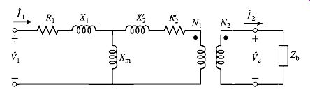
FIG. 21 Equivalent circuit for an instrumentation transformer.

Consider first a potential transformer. Ideally it should accurately measure voltage while appearing as an open circuit to the system under measurement, i.e., drawing negligible current and power. Thus, its load impedance should be "large" in a sense we will now quantify.

First, let us assume that the transformer secondary is open-circuited. In this case we can write that ...

(EQN. 41)

From this equation, we see that a potential transformer with an open-circuited secondary has an inherent error (in both magnitude and phase) due to the voltage drop of the magnetizing current through the primary resistance and leakage reactance. To the extent that the primary resistance and leakage reactance can be made small compared to the magnetizing reactance, this inherent error can be made quite small.

The situation is worsened by the presence of a finite burden. Including the effect of the burden impedance, Eq. 41 becomes ....

(EQN. 42)

(EQN. 43)

(EQN. 44)

... is the burden impedance referred to the transformer primary.

From these equations, it can be seen that the characteristics of an accurate potential transformer include a large magnetizing reactance (more accurately, a large exciting impedance since the effects of core loss, although neglected in the analysis presented here, must also be minimized) and relatively small winding resistances and leakage reactances. Finally, as will be seen in Example 10, the burden impedance must be kept above a minimum value to avoid introducing excessive errors in the magnitude and phase angle of the measured voltage.

Consider next a current transformer. An ideal current transformer would accurately measure voltage while appearing as a short circuit to the system under measurement, i.e., developing negligible voltage drop and drawing negligible power. Thus, its load impedance should be "small" in a sense we will now quantify.

Let us begin with the assumption that the transformer secondary is short-circuited. In this case we can write that ...

(EQN. 45)

In a fashion quite analogous to that of a potential transformer, Eq. 45 shows that a current transformer with a shorted secondary has an inherent error (in both magnitude and phase) due to the fact that some of the primary current is shunted through the magnetizing reactance and does not reach the secondary. To the extent that the magnetizing reactance can be made large in comparison to the secondary resistance and leakage reactance, this error can be made quite small.

A finite burden appears in series with the secondary impedance and increases the error. Including the effect of the burden impedance, Eq. 45 becomes

(EQN. 46)

From these equations, it can be seen that an accurate current transformer has a large magnetizing impedance and relatively small winding resistances and leakage reactances. In addition, as is seen in Example 11, the burden impedance on a current transformer must be kept below a maximum value to avoid introducing excessive additional magnitude and phase errors in the measured current.

9. THE PER-UNIT SYSTEM

Computations relating to machines, transformers, and systems of machines are often carried out in per-unit form, i.e., with all pertinent quantities expressed as decimal fractions of appropriately chosen base values. All the usual computations are then carried out in these per unit values instead of the familiar volts, amperes, ohms, and so on.

There are a number of advantages to the system. One is that the parameter values of machines and transformers typically fall in a reasonably narrow numerical range when expressed in a per-unit system based upon their rating. The correctness of their values is thus subject to a rapid approximate check. A second advantage is that when transformer equivalent-circuit parameters are converted to their per-unit values, the ideal transformer turns ratio becomes 1:1 and hence the ideal transformer can be eliminated. This greatly simplifies analyses since it eliminates the need to refer impedances to one side or the other of transformers. For complicated systems involving many transformers of different turns ratios, this advantage is a significant one in that a possible cause of serious mistakes is removed.

Quantifies such as voltage V, current I, power P, reactive power Q, voltamperes VA, resistance R, reactance X, impedance Z, conductance G, susceptance B, and admittance Y can be translated to and from per-unit form as follows:

(EQN. 47)

…where "Actual quantity" refers to the value in volts, amperes, ohms, and so on. To a certain extent, base values can be chosen arbitrarily, but certain relations between them must be observed for the normal electrical laws to hold in the per-unit system.

Thus, for a single-phase system,

(EQN. 48)

(EQN. 49)

The net result is that only two independent base quantities can be chosen arbitrarily; the remaining quantities are determined by the relationships of Eqs. 48 and 49. In typical usage, values of VA_base and V_base are chosen first; values of/base and all other quantities in Eqs. 48 and 49 are then uniquely established.

The value of VA_base must be the same over the entire system under analysis.

When a transformer is encountered, the values of gbase differ on each side and should be chosen in the same ratio as the turns ratio of the transformer. Usually the rated or nominal voltages of the respective sides are chosen. The process of referring quantities to one side of the transformer is then taken care of automatically by using Eqs. 48 and 49 in finding and interpreting per-unit values.

This can be seen with reference to the equivalent circuit of Fig. 10c. If the base voltages of the primary and secondary are chosen to be in the ratio of the turns of the ideal transformer, the per-unit ideal transformer will have a unity turns ratio and hence can be eliminated.

If these rules are followed, the procedure for performing system analyses in per-unit can be summarized as follows:

1. Select a VA base and a base voltage at some point in the system.

2. Convert all quantities to per unit on the chosen VA base and with a voltage base that transforms as the turns ratio of any transformer which is encountered as one moves through the system.

3. Perform a standard electrical analysis with all quantities in per unit.

4. When the analysis is completed, all quantities can be converted back to real units (e.g., volts, amperes, watts, etc.) by multiplying their per-unit values by their corresponding base values.

When only one electric device, such as a transformer, is involved, the device's own rating is generally used for the volt-ampere base. When expressed in per-unit form on their rating as a base, the characteristics of power and distribution transformers do not vary much over a wide range of ratings. For example, the exciting current is usually between 0.02 and 0.06 per unit, the equivalent resistance is usually between 0.005 and 0.02 per unit (the smaller values applying to large transformers), and the equivalent reactance is usually between 0.015 and 0.10 per unit (the larger values applying to large high-voltage transformers). Similarly, the per-unit values of synchronous and induction-machine parameters fall within a relatively narrow range. The reason for this is that the physics behind each type of device is the same and, in a crude sense, they can each be considered to be simply scaled versions of the same basic device. As a result, when normalized to their own rating, the effect of the scaling is eliminated and the result is a set of per-unit parameter values which is quite similar over the whole size range of that device.

Often, manufacturers supply device parameters in per unit on the device base.

When several devices are involved, however, an arbitrary choice of volt-ampere base must usually be made, and that value must then be used for the overall system. As a result, when performing a system analysis, it may be necessary to convert the supplied per-unit parameter values to per-unit values on the base chosen for the analysis.

The following relations can be used to convert per-unit (pu) values from one base to another:

(EQN. 50)

(EQN. 51)

(EQN. 52)

(EQN. 53)

10. SUMMARY

Although not an electromechanical device, the transformer is a common and indispensable component of ac systems where it is used to transform voltages, currents, and impedances to appropriate levels for optimal use. For the purposes of our study of electromechanical systems, transformers serve as valuable examples of the analysis techniques which must be employed. They offer us opportunities to investigate the properties of magnetic circuits, including the concepts of mmf, magnetizing current, and magnetizing, mutual, and leakage fluxes and their associated inductances.

In both transformers and rotating machines, a magnetic field is created by the combined action of the currents in the windings. In an iron-core transformer, most of this flux is confined to the core and links all the windings. This resultant mutual flux induces voltages in the windings proportional to their number of turns and is responsible for the voltage-changing property of a transformer. In rotating machines, the situation is similar, although there is an air gap which separates the rotating and stationary components of the machine. Directly analogous to the manner in which transformer core flux links the various windings on a transformer core, the mutual flux in rotating machines crosses the air gap, linking the windings on the rotor and stator.

As in a transformer, the mutual flux induces voltages in these windings proportional to the number of turns and the time rate of change of the flux.

A significant difference between transformers and rotating machines is that in rotating machines there is relative motion between the windings on the rotor and stator.

This relative motion produces an additional component of the time rate of change of the various winding flux linkages. As will be discussed in Section 3, the resultant voltage component, known as the speed voltage, is characteristic of the process of electromechanical energy conversion. In a static transformer, however, the time variation of flux linkages is caused simply by the time variation of winding currents; no mechanical motion is involved, and no electromechanical energy conversion takes place.

The resultant core flux in a transformer induces a counter emf in the primary which, together with the primary resistance and leakage-reactance voltage drops, must balance the applied voltage. Since the resistance and leakage-reactance voltage drops usually are small, the counter emf must approximately equal the applied voltage and the core flux must adjust itself accordingly. Exactly similar phenomena must take place in the armature windings of an ac motor; the resultant air-gap flux wave must adjust itself to generate a counter emf approximately equal to the applied voltage.

In both transformers and rotating machines, the net mmf of all the currents must accordingly adjust itself to create the resultant flux required by this voltage balance.

In any ac electromagnetic device in which the resistance and leakage-reactance voltage drops are small, the resultant flux is very nearly determined by the applied voltage and frequency, and the currents must adjust themselves accordingly to produce the mmf required to create this flux.

In a transformer, the secondary current is determined by the voltage induced in the secondary, the secondary leakage impedance, and the electric load. In an induction motor, the secondary (rotor) current is determined by the voltage induced in the secondary, the secondary leakage impedance, and the mechanical load on its shaft.

Essentially the same phenomena take place in the primary winding of the transformer and in the armature (stator) windings of induction and synchronous motors. In all three, the primary, or armature, current must adjust itself so that the combined mmf of all currents creates the flux required by the applied voltage.

In addition to the useful mutual fluxes, in both transformers and rotating machines there are leakage fluxes which link individual windings without linking others. Although the detailed picture of the leakage fluxes in rotating machines is more complicated than that in transformers, their effects are essentially the same. In both, the leakage fluxes induce voltages in ac windings which are accounted for as leakage-reactance voltage drops. In both, the reluctances of the leakage-flux paths are dominated by that of a path through air, and hence the leakage fluxes are nearly linearly proportional to the currents producing them. The leakage reactances therefore are often assumed to be constant, independent of the degree of saturation of the main magnetic circuit.

Further examples of the basic similarities between transformers and rotating machines can be cited. Except for friction and windage, the losses in transformers and rotating machines are essentially the same. Tests for determining the losses and equivalent circuit parameters are similar: an open-circuit, or no-load, test gives information regarding the excitation requirements and core losses (along with friction and windage losses in rotating machines), while a short-circuit test together with dc resistance measurements gives information regarding leakage reactances and winding resistances. Modeling of the effects of magnetic saturation is another example: In both transformers and ac rotating machines, the leakage reactances are usually assumed to be unaffected by saturation, and the saturation of the main magnetic circuit is assumed to be determined by the resultant mutual or air-gap flux.

11. PROBLEMS

1. A transformer is made up of a 1200-turn primary coil and an open-circuited 75-turn secondary coil wound around a closed core of cross-sectional area 42 cm^2. The core material can be considered to saturate when the rms applied flux density reaches 1.45 T. What maximum 60-Hz rms primary voltage is possible without reaching this saturation level? What is the corresponding secondary voltage? How are these values modified if the applied frequency is lowered to 50 Hz?

2. A magnetic circuit with a cross-sectional area of 15 cm^2 is to be operated at 60 Hz from a 120-V rms supply. Calculate the number of turns required to achieve a peak magnetic flux density of 1.8 T in the core.

3. A transformer is to be used to transform the impedance of a 8-ohm resistor to an impedance of 75 ft. Calculate the required turns ratio, assuming the transformer to be ideal.

4. A 100-fl resistor is connected to the secondary of an idea transformer with a turns ratio of 1:4 (primary to secondary). A 10-V rms, 1-kHz voltage source is connected to the primary. Calculate the primary current and the voltage across the 100-f2 resistor.

5. A source which can be represented by a voltage source of 8 V rms in series with an internal resistance of 2 k Ohm is connected to a 50-f2 load resistance through an ideal transformer. Calculate the value of turns ratio for which maximum power is supplied to the load and the corresponding load power? Using MATLAB, plot the power in milliwatts supplied to the load as a function of the transformer ratio, covering ratios from 1.0 to 10.0.

6. Repeat Problem 5 with the source resistance replaced by a 2-kf2 reactance.

7. A single-phase 60-Hz transformer has a nameplate voltage rating of 7.97 kV:266 V, which is based on its winding turns ratio. The manufacturer calculates that the primary (7.97-kV) leakage inductance is 165 mH and the primary magnetizing inductance is 135 H. For an applied primary voltage of 7970 V at 60 Hz, calculate the resultant open-circuit secondary voltage.

8. The manufacturer calculates that the transformer of Problem 7 has a secondary leakage inductance of 0.225 mH.

a. Calculate the magnetizing inductance as referred to the secondary side.

b. A voltage of 266 V, 60 Hz is applied to the secondary. Calculate (i) the resultant open-circuit primary voltage and (ii) the secondary current which would result if the primary were short-circuited.

9. A 120-V:2400-V, 60-Hz, 50-kVA transformer has a magnetizing reactance (as measured from the 120-V terminals) of 34.6 ft. The 120-V winding has a leakage reactance of 27.4 mr^2 and the 2400-V winding has a leakage reactance of 11.2 ft.

a. With the secondary open-circuited and 120 V applied to the primary (120-V) winding, calculate the primary current and the secondary voltage.

b. With the secondary short-circuited, calculate the primary voltage which will result in rated current in the primary winding. Calculate the corresponding current in the secondary winding.

10. A 460-V:2400-V transformer has a series leakage reactance of 37.2 f^2 as referred to the high-voltage side. A load connected to the low-voltage side is observed to be absorbing 25 kW, unity power factor, and the voltage is measured to be 450 V. Calculate the corresponding voltage and power factor as measured at the high-voltage terminals.

11. The resistances and leakage reactances of a 30-kVA, 60-Hz, 2400-V:240-V distribution transformer are

R1 = 0.68 f2 R2 = 0.0068 f^2

X11 = 7.8 f2 X12 = 0.0780

where subscript 1 denotes the 2400-V winding and subscript 2 denotes the 240-V winding. Each quantity is referred to its own side of the transformer.

a. Draw the equivalent circuit referred to (i) the high- and (ii) the low-voltage sides. Label the impedances numerically.

b. Consider the transformer to deliver its rated kVA to a load on the low-voltage side with 230 V across the load. (i) Find the high-side terminal voltage for a load power factor of 0.85 power factor lagging. (ii) Find the high-side terminal voltage for a load power factor of 0.85 power factor leading.

c. Consider a rated-kVA load connected at the low-voltage terminals operating at 240V. Use MATLAB to plot the high-side terminal voltage as a function of the power-factor angle as the load power factor varies from 0.6 leading through unity power factor to 0.6 pf lagging.

12. Repeat Problem 11 for a 75-kVA, 60-Hz, 4600-V:240-V distribution transformer whose resistances and leakage reactances are

R1 = 0.846 f2 R2 = 0.00261

X~ = 26.8 f2 X12 = 0.0745 f2

where subscript 1 denotes the 4600-V winding and subscript 2 denotes the 240-V winding. Each quantity is referred to its own side of the transformer.

13. A single-phase load is supplied through a 35-kV feeder whose impedance is 95 + j360 f2 and a 35-kV:2400-V transformer whose equivalent impedance is:

0.23 + j 1.27 f2 referred to its low-voltage side. The load is 160 kW at 0.89 leading power factor and 2340 V.

a. Compute the voltage at the high-voltage terminals of the transformer.

b. Compute the voltage at the sending end of the feeder.

c. Compute the power and reactive power input at the sending end of the feeder.

14. Repeat Example 6 with the transformer operating at full load and unity power factor.

15. The nameplate on a 50-MVA, 60-Hz single-phase transformer indicates that it has a voltage rating of 8.0-kV:78-kV. An open-circuit test is conducted from the low-voltage side, and the corresponding instrument readings are 8.0 kV, 62.1 A, and 206 kW. Similarly, a short-circuit test from the low-voltage side gives readings of 674 V, 6.25 kA, and 187 kW.

a. Calculate the equivalent series impedance, resistance, and reactance of the transformer as referred to the low-voltage terminals.

b. Calculate the equivalent series impedance of the transformer as referred to the high-voltage terminals.

c. Making appropriate approximations, draw a T equivalent circuit for the transformer.

d. Determine the efficiency and voltage regulation if the transformer is operating at the rated voltage and load (unity power factor).

e. Repeat part (d), assuming the load to be at 0.9 power factor leading.

16. A 550-kVA, 60-Hz transformer with a 13.8-kV primary winding draws 4.93 A and 3420 W at no load, rated voltage and frequency. Another transformer has a core with all its linear dimensions ~ times as large as the corresponding dimensions of the first transformer. The core material and lamination thickness are the same in both transformers. If the primary windings of both transformers have the same number of turns, what no-load current and power will the second transformer draw with 27.6 kV at 60 Hz impressed on its primary?

17. The following data were obtained for a 20-kVA, 60-Hz, 2400:240-V distribution transformer tested at 60 Hz:

a. Compute the efficiency at full-load current and the rated terminal voltage at 0.8 power factor.

b. Assume that the load power factor is varied while the load current and secondary terminal voltage are held constant. Use a phasor diagram to determine the load power factor for which the regulation is greatest. What is this regulation?

18. A 75-kVa, 240-V:7970-V, 60-Hz single-phase distribution transformer has the following parameters referred to the high-voltage side:

R1 = 5.93 f2 X1 = 43.2

R2 = 3.39 f2 X2 = 40.6 f2

Rc = 244 kf2 X m = 114 k~

Assume that the transformer is supplying its rated kVA at its low-voltage terminals. Write a MATLAB script to determine the efficiency and regulation of the transformer for any specified load power factor (leading or lagging). You may use reasonable engineering approximations to simplify your analysis. Use your MATLAB script to determine the efficiency and regulation for a load power factor of 0.87 leading.

19. The transformer of Problem 11 is to be connected as an autotransformer.

Determine (a) the voltage ratings of the high- and low-voltage windings for this connection and (b) the kVA rating of the autotransformer connection.

20. A 120:480-V, 10-kVA transformer is to be used as an autotransformer to supply a 480-V circuit from a 600-V source. When it is tested as a two-winding transformer at rated load, unity power factor, its efficiency is 0.979.

a. Make a diagram of connections as an autotransformer.

b. Determine its kVA rating as an autotransformer.

c. Find its efficiency as an autotransformer at full load, with 0.85 power factor lagging.

21. Consider the 8-kV:78-kV, 50-MVA transformer of Problem 15 connected as an autotransformer.

a. Determine the voltage ratings of the high- and low-voltage windings for this connection and the kVA rating of the autotransformer connection.

b. Calculate the efficiency of the transformer in this connection when it is supplying its rated load at unity power factor.

22. Write a MATLAB script whose inputs are the rating (voltage and kVA) and rated-load, unity-power-factor efficiency of a single-transformer and whose output is the transformer rating and rated-load, unity-power-factor efficiency when connected as an autotransformer.

23. The high-voltage terminals of a three-phase bank of three single-phase transformers are supplied from a three-wire, three-phase 13.8-kV (line-to-line) system. The low-voltage terminals are to be connected to a three-wire, three-phase substation load drawing up to 4500 kVA at 2300 V line-to-line.

Specify the required voltage, current, and kVA ratings of each transformer (both high- and low-voltage windings) for the following connections:

24. Three 100-MVA single-phase transformers, rated at 13.8 kV:66.4 kV, are to be connected in a three-phase bank. Each transformer has a series impedance of 0.0045 + j0.19 f2 referred to its 13.8-kV winding.

a. If the transformers are connected Y-Y, calculate (i) the voltage and power rating of the three-phase connection, (ii) the equivalent impedance as referred to its low-voltage terminals, and (iii) the equivalent impedance as referred to its high-voltage terminals.

b. Repeat part (a) if the transformer is connected Y on its low-voltage side and A on its high-voltage side.

25. Repeat Example 8 for a load drawing rated current from the transformers at unity power factor.

26. A three-phase Y-A transformer is rated 225-kV:24-kV, 400 MVA and has a series reactance of 11.7 f2 as referred to its high-voltage terminals. The transformer is supplying a load of 325 MVA, with 0.93 power factor lagging at a voltage of 24 kV (line-to-line) on its low-voltage side. It is supplied from a feeder whose impedance is 0.11 + j 2.2 f2 connected to its high-voltage terminals. For these conditions, calculate (a) the line-to-line voltage at the high-voltage terminals of the transformer and (b) the line-to-line voltage at the sending end of the feeder.

27. Assume the total load in the system of Problem 26 to remain constant at 325 MVA. Write a MATLAB script to plot the line-to-line voltage which must be applied to the sending end of the feeder to maintain the load voltage at 24 kV line-to-line for load power factors in range from 0.75 lagging to unity to 0.75 leading. Plot the sending-end voltage as a function of power factor angle.

28. A A-Y-connected bank of three identical 100-kVA, 2400-V: 120-V, 60-Hz transformers is supplied with power through a feeder whose impedance is 0.065 + j0.87 f2 per phase. The voltage at the sending end of the feeder is held constant at 2400 V line-to-line. The results of a single-phase short-circuit test on one of the transformers with its low-voltage terminals short-circuited are

VH=53.4V

f=60Hz

IH=41.7A

P=832W

a. Determine the line-to-line voltage on the low-voltage side of the transformer when the bank delivers rated current to a balanced three-phase unity power factor load.

b. Compute the currents in the transformer's high- and low-voltage windings and in the feeder wires if a solid three-phase short circuit occurs at the secondary line terminals.

29. A 7970-V: 120-V, 60-Hz potential transformer has the following parameters as seen from the high-voltage (primary) winding:

a. Assuming that the secondary is open-circuited and that the primary is connected to a 7.97-kV source, calculate the magnitude and phase angle (with respect to the high-voltage source) of the voltage at the secondary terminals.

b. Calculate the magnitude and phase angle of the secondary voltage if a 1-kfl resistive load is connected to the secondary terminals.

c. Repeat part (b) if the burden is changed to a 1-kf2 reactance.

30. For the potential transformer of Problem 29, find the maximum reactive burden (minimum reactance) which can be applied at the secondary terminals such that the voltage magnitude error does not exceed 0.5 percent.

31 Consider the potential transformer of Problem 29.

a. Use MATLAB to plot the percentage error in voltage magnitude as a function of the magnitude of the burden impedance (i) for a resistive burden of 100 ~2 < Rb < 3000 ~ and (ii) for a reactive burden of 100 g2 < Xb < 3000 f^2. Plot these curves on the same axis.

b. Next plot the phase error in degrees as a function of the magnitude of the burden impedance (i) for a resistive burden of 100 f2 < Rb < 3000 f^2 and (ii) for a reactive burden of 100 f^2 < Xb < 3000 f2. Again, plot these curves on the same axis.

32. A 200-A:5-A, 60-Hz current transformer has the following parameters as seen from the 200-A (primary) winding:

X1 = 745/zg^2

X~ = 813/xg^2

Xm = 307 mr^2

R1 = 136/zf^2

R2 = 128/zf^2

a. Assuming a current of 200 A in the primary and that the secondary is short-circuited, find the magnitude and phase angle of the secondary current.

b. Repeat the calculation of part (a) if the CT is shorted through a 250 #~ burden.

33. Consider the current transformer of Problem 32.

a. Use MATLAB to plot the percentage error in current magnitude as a function of the magnitude of the burden impedance (i) for a resistive burden of 100 f2 < Rb < 1000 f2 and (ii) for a reactive burden of 100 ~ < Xb < 1000 f2. Plot these curves on the same axis.

b. Next plot the phase error in degrees as a function of the magnitude of the burden impedance (i) for a resistive burden of 100 f2 < Rb < 1000 f2 and (ii) for a reactive burden of 100 f2 < Xb < 1000 f2. Again, plot these curves on the same axis.

34. A 15-kV: 175-kV, 125-MVA, 60-Hz single-phase transformer has primary and secondary impedances of 0.0095 + j0.063 per unit each. The magnetizing impedance is j 148 per unit. All quantities are in per unit on the transformer base. Calculate the primary and secondary resistances and reactances and the magnetizing inductance (referred to the low-voltage side) in ohms and henrys.

35. The nameplate on a 7.97-kV:460-V, 75-kVA, single-phase transformer indicates that it has a series reactance of 12 percent (0.12 per unit).

a. Calculate the series reactance in ohms as referred to (i) the low-voltage terminal and (ii) the high-voltage terminal.

b. If three of these transformers are connected in a three-phase Y-Y connection, calculate (i) the three-phase voltage and power rating, (ii) the per unit impedance of the transformer bank, (iii) the series reactance in ohms as referred to the high-voltage terminal, and (iv) the series reactance in ohms as referred to the low-voltage terminal.

c. Repeat part (b) if the three transformers are connected in Y on their HV side and A on their low-voltage side.

36. a. Consider the Y-Y transformer connection of Problem 35, part (b). If the rated voltage is applied to the high-voltage terminals and the three low-voltage terminals are short-circuited, calculate the magnitude of the phase current in per unit and in amperes on (i) the high-voltage side and (ii) the low-voltage side.

b. Repeat this calculation for the Y-A connection of Problem 35, part (c).

37 A three-phase generator step-up transformer is rated 26-kV:345-kV, 850 MVA and has a series impedance of 0.0035 + j0.087 per unit on this base. It is connected to a 26-kV, 800-MVA generator, which can be represented as a voltage source in series with a reactance of j 1.57 per unit on the generator base.

a. Convert the per unit generator reactance to the step-up transformer base.

b. The unit is supplying 700 MW at 345 kV and 0.95 power factor lagging to the system at the transformer high-voltage terminals. (i) Calculate the transformer low-side voltage and the generator internal voltage behind its reactance in kV. (ii) Find the generator output power in MW and the power factor.