AMAZON multi-meters discounts AMAZON oscilloscope discounts
1. Introduction
Measurement is an activity which pervades almost all human endeavors. In industrial countries about 5 percent of the gross national product is devoted to making measurements and this figure is comparable with the expenditure on the health services in the UK. Three major areas of the use of measurement and instrumentation are in product manufacture, in the process industries and in the exchange of commodities.
Measurement by means of instruments takes place at all stages of the manufacturing process from the validation of bought-in components, through the assessment of the process, in safety tests and environmental tests and in the final check of conformance with the customer's specification. Measurement is the arbiter of quality - the ability to meet the customer's needs.
Instruments pervade the process industries where flow, temperature, pressure and liquid level are very commonly measured quantities. The ability to control these quantities depends on the ability to measure the quantities satisfactorily. Thus measurement, often by means of a sensor, is found in every control loop of the process.
When commodities change hands, from pears to petroleum, acceptable measurement is the dispenser of fair play. A traditional role of government is to ensure the availability of an accepted system of measurement for trade throughout the country.
When some property of an object is measured a number is assigned to the property in terms of the agreed unit value in such a way that the number faithfully reflects the characteristics of the property. This is a definition of measurement. In producing a number which reflects the property, the quantity (how much?) of the quality (of what sort?) is obtained. In order that the number does reflect the property in question, it is essential that the influence of other qualities is kept to a minimum. An ideal measurement would therefore be one for which the result is only affected by the size of the quantity to be measured and by no other. Much effort in designing and using instruments goes into meeting this condition of satisfactory measurement as closely as possible.
It is clear from the above that the subject of measurement and instrumentation is a vast one. Restricting the subject to electrical engineering is in fact not much of a restriction as very many non-electrical measurements are converted into electrical measurements via suitable sensors, owing to the accuracy and convenience of electrical measurement. It is therefore impossible to cover this subject completely, nor is it necessary. By describing the major instruments - the Cathode Ray OsciUoscope (CRO), the Digital Storage Oscilloscope (DSO), the frequency counter, the Digital Voltmeter (DVM), the Digital Multimeter (DMM) and some important sensors -the principles and practice of measurement and instrumentation can be outlined.
2. The oscilloscope
The most commonly used instrument in electronic and electrical engineering is the cathode ray oscilloscope or its digital counterpart, the digital storage oscilloscope. It is difficult to envisage design, development, testing or maintenance without the oscilloscope. The oscilloscope makes visible the waveforms in the circuits of interest and is therefore the means whereby the engineer can bring his knowledge, experience and creativity to bear on the situation.
2.1 The cathode ray oscilloscope
The CRO is an instrument which presents to the engineer a 'graph' of the voltage signal at a point in a circuit against time, as shown in Fig. 1. This is a very helpful form of presentation for the engineer since this is the way in which signals are conceived. It is possible to measure both time and amplitude information with such a display. The display can be used quantitatively to investigate, for example, waveform distortion. How this is achieved can be seen by a consideration of the construction of the CRO.
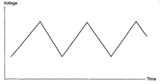
Fig. 1 The CRO display
Figure 2 shows a simplified diagram of a Cathode Ray Tube (CRT). The CRT is at the heart of the CRO. It consists of an indirectly heated cathode which is coated with a material capable of giving a large number of electrons when heated. The electrons are attracted away from the vicinity of the cathode by the anode which is at a high positive voltage. By careful design the electrons pass along the tube and hit the phosphor coating inside the CRT screen. Phosphor is the name of a family of materials that possess fluorescence and phosphorescence. Fluorescence is the property of a material to give off light when struck by the fast moving electrons. Phosphorescence is the property of a material to keep giving off light for some time after having been struck by the electrons. The time for which the light is given out is the persistence of the phosphor. CROs are supplied with either general purpose or long persistence phosphors. General purpose phosphors have persistence of the order of tens of milliseconds and long persistence phosphors have persistence of the order of a few seconds. A long persistence phosphor is advantageous for a very low frequency waveform, perhaps less than 1 Hz, as the whole waveform can be seen by means of the long period of phosphorescence. However, long persistence phosphors are easily damaged by, for example, allowing the electron beam to be stationary for some time.
Most CROs therefore have general purpose phosphors.
The deflection of the electron beam in order to display the applied signal is achieved very directly in the CRO by applying a scaled version of the signal to the deflection plates. The relationship between the deflection and the applied voltage is a linear one and so the interpretation of the resulting display is an easy matter.
In order for the display on the CRO screen to look like a graph of the signal it is necessary to have uniformly increasing horizontal deflection as well as the vertical signal deflection described. A linearly rising voltage applied to the X deflection plates achieves this. To obtain an easily viewed display of a repetitive signal, it is usual for internal circuitry to produce a repeated sweep from left to right. The waveform which achieves this is called a saw-tooth waveform and is shown in Fig. 3.
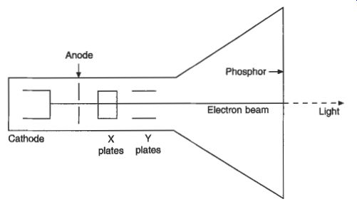
Fig. 2 Cathode ray tube construction
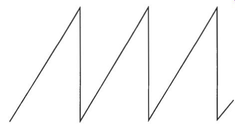
Fig. 3 The saw-tooth waveform
2.2 The steady display of a repetitive signal
To obtain a usable display, it is clearly necessary for the frequencies of the timebase and the input frequency to be simply related, such as 1 : 1, 1 : 2, 1 : 3 etc. This presents some difficulty since the frequency of the input waveform will probably be unknown until viewed on the CRO. To overcome this, a variable timebase frequency control is provided on the CRO front panel. When this is adjusted to bring the timebase frequency close to a simple relationship with that of the input frequency, internal circuitry locks the timebase frequency to the exact relationship. The display on the screen will therefore be that of one period of the input signal for a 1 : 1 ratio, two periods of the input signal for a 2 : 1 ratio and so on. Thus a steady display of the input signal is provided for signals over a very wide frequency range. Parameters of interest such as period and amplitude can be measured conveniently. An example of a 1 : 1 ratio is shown in Fig. 4. This is called the synchronized method of display.
It often happens, however, that the engineer would like to look at only a small part of the period of a repetitive waveform. Figure 5 shows a sinusoidal type input, but with a ripple on each maximum positive excursion. The synchronized method for signal display shown earlier will not allow the detailed examination of the ripple area of interest, but the trigger method will. In the internal trigger method, a variable dc voltage is set by a control on the front panel. This trigger level voltage is compared with the input signal and one sweep of the timebase is enabled when the input signal exceeds the trigger level. The timebase runs for a time set by the front panel and is in no way related to the value of the input signal. After the sweep, the spot is blanked, flies back and waits for the next occasion when the input exceeds the trigger level.
At this time another sweep occurs and so the display is that of the repetition of the same portion of the waveform again and again. By suitable adjustment of the trigger level and the timebase sweep rate, a small detail can be investigated easily as shown in Fig. 5.
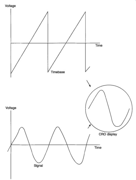
Fig. 4 CRO display for 1 : 1 ratio of timebase and input frequency
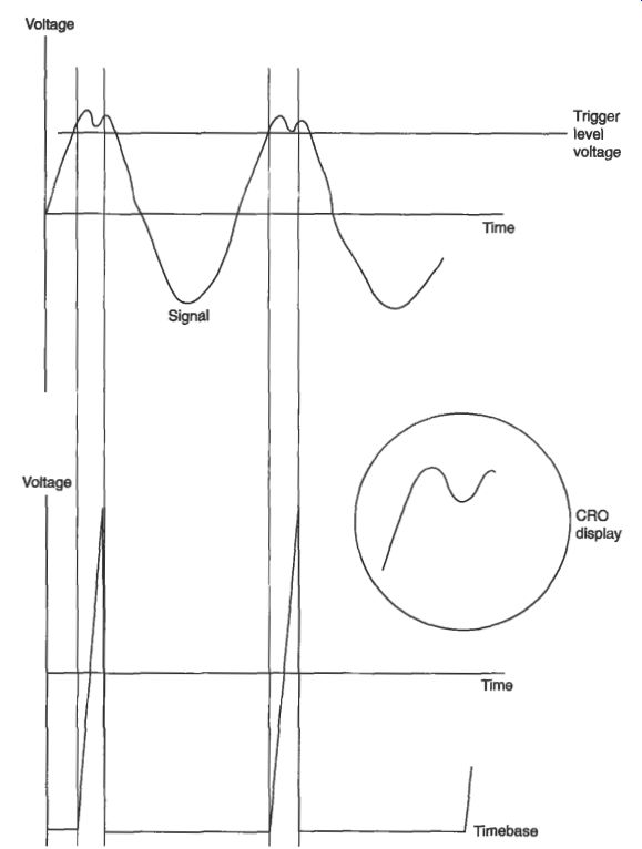
Fig. 5 Trigger method for display of part of a waveform
2.3 The display of one signal against another - Lissajous figures
A CRO can be configured to display one signal against another externally provided signal rather than against the internally provided timebase signal. The ensuing displays are called Lissajous figures after the nineteenth-century Frenchman who investigated the effect of the combination of simple harmonic motions. The method can be very useful for measuring phase shift in a circuit (the concept of phase angle in an ac circuit has been explained in section 2.3.2). Figure 6 shows a linear circuit supplied by a sinusoidal voltage source. The output must also be sinusoidal, but the amplitude and phase will be different from that of the applied input. If the input signal is displayed on the horizontal axis and the output signal is displayed on the vertical axis, then a display such as Fig. 7 occurs. The display can be used to measure the gain, which is the maximum to minimum vertical excursion divided by the maximum to minimum horizontal excursion, yJxg, taking into account the scaling of the x and y controls. More useful, however, is the phase measurement capability. If the horizontal deflection signal is u, = V, sin wt and the vertical deflection signal is uy = Vv sin(m + 4) then the phase shift Q, can be found by the following: at t = 0, v, = 0 u,. = Vy sin(0 + Q,) = V, therefore Expressed in words the phase shift between two signals (such as the input and the output in Fig. 6) can be measured by taking the ratio of the maximum y excursion and the intercept on the x axis and then performing the inverse sine operation. In this way it is easy to observe the phase shift in, for example, an amplifier and to explore how the phase shift changes with frequency.
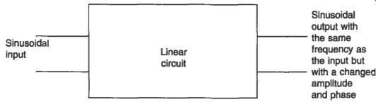
Fig. 6
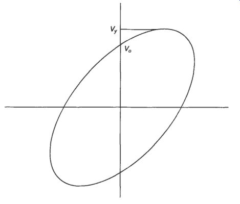
Fig. 7 A Lissajous figure
2.4 The display of two signals against time
Very often it is helpful to be able to observe the waveform and make measurements at two points in a circuit simultaneously. This allows the assessment of the performance of the circuit, for example the distortion introduced by an audio amplifier. In order to do this without significantly increasing the cost of the CRO, then one electron beam must write both signals. Provided this is carefully done, the eye does not see this, but sees two traces simultaneously.
There are two ways of achieving this and most CROs provide both, often automatically switching between the two to suit the frequency of the signal. The two ways are called the alternate method and the chop method. The effect of the alternate method is shown in Fig. 8. In the alternate method, a sweep of the timebase is traced with alternately one input then the other connected to the Y deflection plates.
The two inputs y1 and y2 have their own gain controls and Y deflection controls. This method works well provided the input signal frequency is not too low. For low frequencies, it becomes evident to the eye that the display consists of one trace followed by another.
For low frequencies the chop method is appropriate, and the effect of this is shown in Fig. 9. An internal oscillator running at about 500 kHz is used to switch the two inputs in small sections to the deflection plates. For low-frequency signals, there are very many sections for a sweep, for example 5000 for a 100 Hz signal, and the display appears continuous. At high frequencies, the sectional nature becomes very evident to the eye and the alternate method is used.
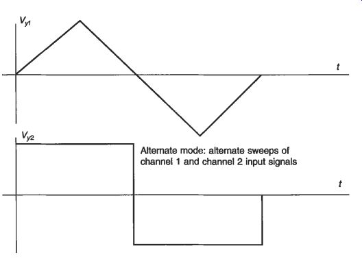
Fig. 8 The alternate mode --- Alternate mode: alternate sweeps of channel
1 and channel 2 input signals
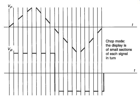
Fig. 9 Display of two ?: inputs in the chop mode
2.5 The ac-dc switch
There are applications where it is desirable to be able to measure the characteristics of a small varying quantity superimposed on a large de value. A typical case would be the assessment of residual ripple on a dc power supply. The CRO has an ac/dc switch on the front panel and in the dc position, the displayed waveform would look like Fig. 10(a). If the sensitivity of the CRO is increased by changing the gain switch, the trace would disappear from the screen. In order to be able to view an enlarged version of the ac component, the switch should be set in the ac position.
This introduces a logical capacitor in series with the signal, blocking the dc component.
The display then looks like Fig. 10(b). It is possible in this position to increase the sensitivity as desired to view the ac quantity. If the displayed signal is very low in frequency, say a few Hz, much of the signal will also be effectively blocked by the capacitor in the ac position and a much reduced amplitude of display will result. For this reason the ac/dc switch should be kept in the dc position for general use.
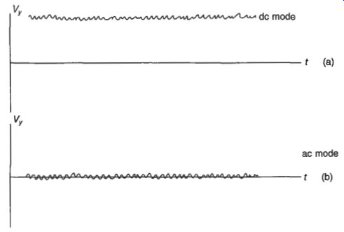
Fig. 10 The effect of the ac/& switch
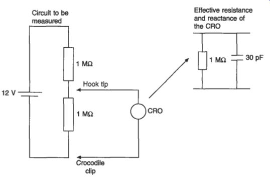
Fig. 11 CRO loading effect
2.6 The loading effect of the CRO
In common with all instruments, the CRO affects the condition of the circuit to which it is connected. This always happens and it is important to discover whether this effect is significant or not. It is called the loading effect of the instrument. A manufacturer will state, usually by the Y input socket, the effective resistance and capacitance of the CRO. The effect of the CRO on the circuit is as if it were a parallel resistor and capacitor, shown in Fig. 11, with typical values for resistance and capacitance shown. As an example a simple potential divider circuit is shown in Fig. 11. Before connecting the CRO, the voltage across the lower 1 M-ohm resistor is 6 V pk-pk by symmetry. When the CRO is connected in the case of low frequencies for which the capacitive effect of the CRO can be neglected, the 1 M-ohm of the CRO reduces the lower resistance to a combined resistance of 1/2 MR. This means that the voltage across the lower resistance will fall to 4 V pk-pk and this is what a perfectly accurate CRO will read. Of course the voltage will return to 6 V pk-pk when the CRO is removed. The effect of the CRO on the circuit is clearly very significant and the effect becomes worse at high frequencies, where the effect of the capacitance of the CRO is to lower further the impedance of the instrument.
If the characteristics of the circuit and the CRO are known, as in the situation shown in Fig. 11, then it is possible to calculate the effect of the loading and correct for it. Usually, however, the CRO is the means of investigating the circuit and no such previous knowledge will be available. The loading effect will only be serious where the impedance of the circuit approaches the impedance of the CRO and it can usually be neglected if the circuit impedance is not greater than one-tenth of the CRO impedance. There are many cases where this condition is not met or it is not known if it is met. The solution is to use a suitable probe with the CRO.
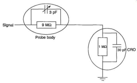
Fig. 12 The use of the x10 probe
2.7 CRO probes
In the body of a typical CRO probe is mounted a switch labeled xl and x10. In the xl position the signal is passed directly to the CRO. In the x10 position a 9 M-ohm resistor and variable parallel capacitor are switched in series with the signal lead, as shown in Fig. 12. At low frequencies, where the effect of the two capacitances can be neglected, the effect of the x10 switch is to increase the effective CRO resistance to 10 MR thus making the loading effect much less significant. At high frequency, the effect of the probe capacitor reduces the effective capacitance of the instrument.
Cable capacitance makes the effect less predictable than for resistance, but it will also significantly reduce the loading effect at high frequencies.
The effect of the x10 probe will also be to drop nine-tenths of the signal voltage across the probe and so only one-tenth will be presented to the CRO. The amplitude readings of the CRO must be multiplied by 10 to give the signal amplitude, hence the name of the probe.
Other more specialist probes are available to further reduce the loading effect of the CRO, but it is found that for many cases the x10 probe gives a sufficient reduction.
2.8 CRO bandwidth and the measurement of rise time
Probably the most important parameter of the CRO is the bandwidth. The bandwidth gives the maximum frequency for which a faithful display of amplitude takes place.
If a sinusoidal signal above the bandwidth frequency is applied to the CRO, then the displayed amplitude will be smaller than would be the case for the same size input at a lower frequency. This is illustrated in Fig. 13, and it is clear that the instrument calibration can only be used for sinusoids below the bandwidth frequency. This is not the most significant effect of the bandwidth of the CRO. It has a direct bearing on the fastest rising edge of a rapidly changing voltage which can faithfully be displayed on the CRO. The display and measurement of such edges are very important in assessing the digital signals that occur in, for example, computers. A CRO cannot respond instantaneously to a very sudden change in voltage. If a very sudden change is applied, the response of the CRO will look like Fig. 14. The response is usually described by the rise time, the time taken for the response to change from 10 per cent to 90 per cent of the final value. It is found that there is a simple relation between the rise time of the CRO and the CRO bandwidth, which is given by
Bandwidth x Rise time = 0.35
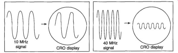
Fig. 13 Effect of a CRO bandwidth of 20 MHz
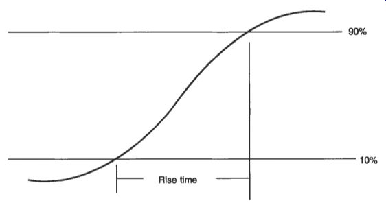
Fig. 14 Response of a CRO to a very fast change in voltage
For example, a 20 MHz CRO will have a rise time of 0.35420 x 10^6) seconds, or 17.5 ns. This means that if the instrument is presented with a voltage waveform with rise times faster than this value, the rise time that will be displayed is the CRO rise time. In order for the effect of the properties of the CRO not to significantly intrude on the display, the fastest rise time that can be displayed should be not less than eight times the CRO rise time. From this relation, the required CRO bandwidth can be calculated in order to display a given signal rise time. For example, if the signal rise time is 80 ns, then the CRO rise time must be 10 ns in order not to change the display significantly. A 10 ns rise time corresponds to a CRO bandwidth of 0.35/10-' Hz, or 35 MHz. This procedure allows the necessary bandwidth to be calculated for a given rise time and checked against the instrument in use, and it can establish whether a new instrument is needed.
Since fast rising voltages are commonly found in digital circuits, the need for high bandwidth CROs is clear.
2.9 The high bandwidth CRO
A high bandwidth CRO is significantly more expensive than a general purpose CRO. There are several reasons for this. In the first place, as the spot moves over the surface very rapidly at high frequencies, the emitted light reduces. To compensate for this the electron beam velocity is increased, but this tends to reduce the sensitivity of the instrument and so extra care is required with the electronics. As the electron beam passes through the deflection plates the forces on the electrons change significantly at high frequencies. This again reduces the sensitivity. This is overcome by splitting the Y deflection plates into a number of small sections arid introducing time delays between each. This ensures that the signal on each plate remains closely the same as the electron beam passes down the tube. It makes the CRT much more expensive, however.
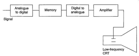
Fig. 15 Y-deflection system in a digital storage oscilloscope
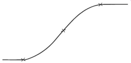
Fig. 16 DSO rise time
2.1 0 The digital storage oscilloscope
The digital storage oscilloscope solves some of the problems of the CRO at high frequencies by means of storing the signal and then displaying at an effective lower frequency. This allows a cheaper CRT to be used. The block diagram of a DSO Y deflection system is shown in Fig. 15. The Analogue to Digital (AD) converter gives a digital version of the voltage input suitable for storing in memory. For the DSO, the CRT ceases to be the critical component at high frequencies. The critical component for the DSO is the AID converter. This element samples the input waveform at regular intervals and converts to a digital equivalent. If the sampling rate is not high enough or the levels of quantization not fine enough, then this will reflect on the accuracy of the quantities measured. An illustration of what happens on a leading voltage edge with a DSO is shown in Fig. 16. The samples are shown by crosses.
This means that the analogue voltage to be measured is converted into numbers at the times shown. The fastest rising edge which can be displayed is when there is one sample on the rising edge. The effective rise time of the DSO is therefore given by 1.6 sample intervals, this is the time from 10 percent to 90 per cent at the final value.
This represents the DSO rise time and a signal should have a slower rise time than this, say six times slower. The fastest acceptable signal rise time is therefore 6 x 1.6 sampling intervals, or lO/sampling rate.
The sampling rate of the DSO is therefore a key parameter of the instrument and is quoted as, for example, 500 M samples per second. Such an instrument is capable of faithfully displaying a signal rise time of 20 ns, and this roughly corresponds to a 140 MHz bandwidth CRO. The other key parameter of the A/D converter is the fineness of quantization, or the number of bits of the A/D. If the number of bits is not sufficiently high, then significant information is lost in the An> process. It is for this reason that a signal displayed on a cheap DSO often appears to have a better signal to noise ratio than for a CRO. The DSO is merely not responding to the small voltage differences of the noise component.
If a good AD converter is used, then the DSO will give a faithful display of an applied signal over a wide range of amplitudes sand frequencies. The DSO has other advantages than cheaper CRT construction. The information in digital form can easily be manipulated to find, for example, average values and rms values. The information can be easily directly communicated to a computer and a hard copy of the display is fairly easily made available.
3. Digital frequency counters, voltmeters and multimeters
Digital multimeters, voltmeters and frequency counters are the next most common instruments used by the electronic and electrical engineer after the CRO and DSO. Since they develop one from the other, the frequency counter will be described first, then the digital voltmeter (DVM) and then the digital multimeter (DMM).
3.1 The frequency counter
The ability to measure accurately the frequency of a signal is a common requirement, for example when designing a filter circuit. This can be achieved by counting the number of periods of the signal that occur in one second, which is the frequency of the signal. The basis of the instrument shown in Fig. 17.
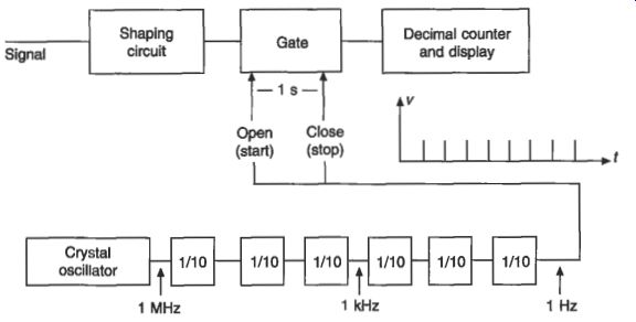
Fig. 17 A frequency counter
The signal is converted into voltage pulses at the same frequency by the shaping circuits, the output from which passes through a gate, is converted into a decimal number, and then shown on a suitable display such as liquid crystal or light emitting diode. The gate is opened for 1 second by arranging that the signal which opens the gate and the signal which closes the gate are derived from a quartz crystal oscillator.
This arrangement works very well for high-frequency signals, since the number of pulses counted is very high, but not so well for a low-frequency signal, for example one with a frequency of 10 Hz.
For such a signal, the +1 error, which occurs for all digital instruments, is a major source of uncertainty in the measurement results. When the number of pulses from the shaping circuit is measured, the gating time is not synchronized with the signal.
It is therefore possible to just miss pulses or just include pulses at either end of the gating period, as shown in Fig. 18. The measured result is therefore 9 Hz and 11 Hz respectively, whereas 10 Hz would be a more representative value. Because of the ever present +1 error in digital instruments, it is important to ensure that the number of pulses counted is very high so that the effect of the f error becomes very small.

Fig. 18 The fl error
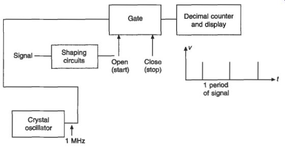
Fig. 19 The period counter
3.1.1 The measurement of low frequencies
For a low-frequency signal, the above condition of ensuring many counted pulses is difficult to achieve. It would be possible to wait for 10 seconds instead of 1 second for the result, which would help a little in reducing the effect of the fl error, but this would still not be acceptable, neither would waiting for 100 seconds. The preferred solution is to swap the signal and crystal oscillator output around as shown in Fig. 19. The signal now opens the gate for exactly one period. The decimal counter will accumulate the number of 1 ps pulses from the crystal oscillator in one period of the signal and the instrument therefore measures the period of the signal. It is clear that the decimal counter will collect a large number of pulses for a low-frequency signal and the fl error will have relatively little effect on the period measurement.
Therefore for a high-frequency signal, frequency measurement should be used and for a low-frequency signal, period measurement should be used. In the case illustrated, it makes no difference for a 1 kHz signal which method is used.
3.1.2 The accuracy of the frequency counter
The potential accuracy of the frequency counter is very high since essentially counting is involved. The key component for the accuracy of the instrument is the crystal oscillator.
The frequency of a crystal depends on many things but usually the temperature, the supply voltage and its age are the three dominant factors. By selecting a crystal cut at a very carefully specified angle to the crystallographic axis, called the AT cut, a quartz crystal with a very low temperature coefficient can be produced. For instruments for which very high accuracy is specified, this crystal is also enclosed in a temperature controlled box. This is more expensive, but gives a very stable frequency with changes in ambient temperature.
The dc supply to the oscillator needs to be carefully controlled in order to avoid frequency changes owing to this cause. A typical figure would be a change of 1 part in lo9 for a 210 per cent change in power supply voltage.
Quartz crystals change their frequency with time after manufacture. In common with many products, the change is most rapid initially and then settles down to a smaller rate of change. A typical characteristic is shown in Fig. 20. From this it can be seen that the initial rate of change might well be significant and recalibration is required more frequently when the instrument is new. This is described in more detail in section 4.5.
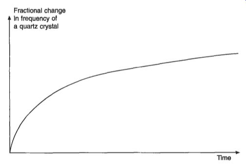
Fig. 20 Change in frequency of a quartz crystal with time
With reasonable care with these matters it is possible to produce a very accurate frequency counter for a modest cost.
3.2 The digital voltmeter
As frequency and time interval can be measured accurately easily and cheaply, it is attractive to make a digital voltmeter (DVM) which converts the dc voltage to be measured to a corresponding time interval or frequency. There are several methods for achieving this and, by way of illustration, the dual slope DVM will be described.
The block diagram for the dual slope DVM and the voltage waveforms are shown in Figs 21 and 22 respectively. At the beginning of the cycle, the unknown voltage is connected to the integrator. The output of an integrator for a dc input is a ramp voltage the slope of which is proportional to the unknown voltage. After one period of the mains supply (20 ms for 50 Hz) the integrator input is switched to an internal stable reference voltage of opposite polarity from that of the voltage to be measured. The output of the integrator then ramps down with a constant slope in all cases. At the same moment as the integrator input is switched, the gate in a timing set-up is opened. This allows pulses from the crystal oscillator to the decimal counter.
This continues until the instant at which the output of the integrator returns to the common voltage, when the gate is closed. The number of pulses counted is directly proportional to the unknown voltage and the display is suitably scaled in volts.
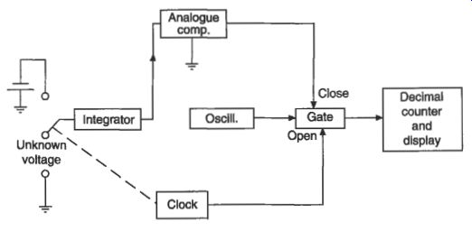
Fig. 21 Dual slope DVM
This method for voltage measurement has several attractions. First, it can be manufactured cheaply. Also mains frequency interference, which must always be present, is eliminated by the integration over one period of the mains. The fact that two slopes are involved means that parameters of the integrator, which change with ambient conditions such as temperature, affect both slopes equally and cancel.
Reasonable accuracy and noise immunity can therefore be achieved by this method.
The accuracy of the digital voltmeter is that of the frequency counter plus the contributions of the extra components, particularly the voltage source and range defining resistors.
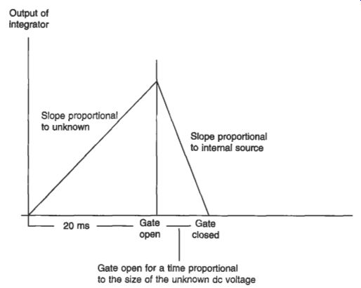
Fig. 22 Timing diagram for the dual slope DVM
3.3 The digital multimeter
The digital multimeter (DMM) is an extension to the digital voltmeter. Just as the digital voltmeter turns the voltage to be measured into a time interval, so the digital multimeter turns the quantity to be measured into a voltage.
Since the digital voltmeter contains a frequency counter, it is possible to provide frequency measurement capabilities directly with modest performance. DC current measurement can be obtained by passing the current to be measured through a resistor and then measuring the voltage developed by the digital voltmeter. The digital multimeter contains a chain of stable resistors which can be selected for various current ranges. The accuracy on the current range will clearly not be as high as for dc voltage. AC voltage can be measured by converting to an equivalent dc voltage. The cheaper schemes rely on rectification and averaging and the calibrations only hold for a sinusoidal signal. More generally used is the true rms converter which gives the nns voltage of the measured quantity regardless of its waveform. The instrument with true rms capability tends to be more expensive.
Resistance measurement can be added in the digital multimeter. The most elegant way of doing this for a dual slope measurement is to pass the same current through the resistor to be measured and a stable reference resistor. The dual slope method can be involved and the voltage across the unknown resistor applied to the integrator of Fig. 21 for the first of the slopes and the voltage across the reference resistor applied to the integrator for the second of the slopes. The time for which the gate is open will be proportional to the unknown resistor and the display can be scaled in ohms. This method is insensitive to changes in the value of current flowing through the resistors, but the stability of the reference resistor is clearly important for the accuracy of the DMM in this mode.
4. Sensors
A sensor is a device which converts the quantity to be measured into another quantity which is easier to present as a number, to manipulate or to display. The human body of course employs sensors, the eye converting optical information, the ear sound information and so on into internal information suitable for further processing. The range of industrial sensors is vast since almost any physical effect relating two quantities can potentially be used as the basis of a sensor. Most conveniently, the output quantity is an electrical one since this makes available the array of tools of signal conditioning and computation.
Sensors can be categorized in a number of ways. Sensors are described as active when energy conversion takes place, such as the piezoelectric sensor converting pressure information into electrical information. Sensors are described as passive when external power is required, such as the rotary potentiometer converting angle into slider voltage when an electrical current flows.
Sensors can be categorized according to the quantity which is changed by the input quantity, such as resistive sensors for measuring temperature of pressure or light intensity or strain or magnetic field.
As always in measurement and instrumentation, the acceptable sensor must give information about the quantity to be measured and be as little sensitive as possible to all other influence quantities. This is by no means easy, since the list of resistive sensors above indicates that, for example, a strain gauge will also change its resistance with temperature, pressure, light intensity, magnetic field and so on. Careful design and intelligence in use is necessary for reliable measurement. The sensor must also be reliable, cheap, not unduly disturb the system to be measured and preferably not involve a major education program on the part of the potential users.
To illustrate from among the vast list of sensors available, three common and typical examples will be described - the strain gauge, the piezoelectric accelerometer and the Linear Variable Differential Transformer (LVDT).
4.1 The strain gauge
A strain gauge is a sensor which converts change in length into a change in resistance and hence voltage. By carefully attaching the strain gauge to the surface of an object, dimensional changes in the object can be monitored and measured. A typical simple strain gauge is shown in Fig. 23. It consists of a metal foil formed into a grid structure by a photo-etching process situated on a resin film. The gauge is designed to have much more conductor along the axis to be measured than at right angles. As the gauge is strained, the resistance changes. The resistance is given by R = pWA where p is the resistivity of the material, L is the length and A the cross-sectional area. All three of these change with strain. For commonly used material the gauge factor, the fractional change in resistance caused by a fractional change in length, is close to 2. Alloys are selected with a low temperature coefficient of resistance and a low temperature coefficient of linear expansion.
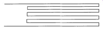
Fig. 23 The strain gauge
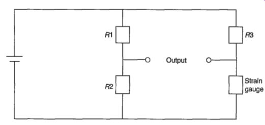
Fig. 24 Strain gauge in a Wheatstone bridge circuit
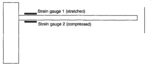
Fig. 25 Strain gauges mounted on a cantilever
If the strain gauge is connected in the Wheatstone bridge circuit shown in Fig. 24, then the output will change as the strain changes. Influence quantities such as temperature will also produce changes in the output. A useful method for significantly reducing these effects is to mount a second gauge in a suitable position. For the measurement of the strain of a cantilever, shown in Fig. 25, then the two gauges will experience dimensional changes which are equal but of opposite sign (one stretched and the other compressed) but equal changes in resistance owing to influence quantities such as temperature. By connecting the gauges to adjacent arms of the Wheatstone bridge circuit, then the unwanted effects tend to cancel, whilst the effect of the change in resistance with strain is doubled.
4.2 The piezoelectric accelerometer
Changes in the vibrations of machinery give information about likely future failure of the equipment, and measurement of vibration using an accelerometer can therefore be used to inform maintenance actions in a cost effective manner. A common way of achieving this is by a piezoelectric accelerometer, shown in Fig. 26. As its name implies, a piezoelectric element converts pressure into an electrical quantity and vice versa. Usually in accelerometers a manufactured ceramic piezoelectric material such as PZT (lead zirconate titanate) is used. Acceleration causes the piezoelectric element to be compressed, thus giving an electrical output which can be used to monitor the acceleration. In a commercial device, care is taken to avoid sensitivity to acceleration in other axes. This is an active device and the output signal in electrical form is generated from the input signal in mechanical form. These types of device are also known as transducers. The piezoelectric accelerometer is usually operated well below its resonance frequency where the output varies little with frequency. There is no dc output from these devices, but when used with a charge amplifier good low-frequency performance can be achieved.
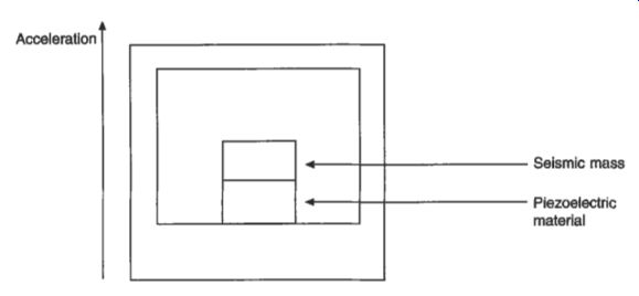
Fig. 26 The piezoelectric accelerometer
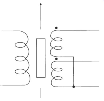
Fig. 27 The LVDT
4.3 The linear variable differential transformer
The LVDT has found widespread acceptance as an industrial displacement sensor.
The construction of the LVDT is shown in Fig. 27. The sensor is a transformer that has a primary and two identical secondary windings which are connected in series opposition. The effect of this is that the output voltage is the difference between the two second voltages. A ferromagnetic rod made from a nickel-iron alloy moves inside the coils and as it moves the output voltage in one coil goes up and the other down. About the centre position, the phase of the signal reverses. LVDTs are made commercially with movement ranges from +-100 pm to +-25 cm.
The LVDT has some attractive features for industrial use. Since there is no mechanical connection between the core and the rest of the instrument friction is low, tolerance to mechanical overload and shock is high and reliability is high. The windings can be set in epoxy resin and the sensor housed in a metal shield thus enabling the LVDT to be used in hostile environments. There is electrical isolation between the primary and secondary windings thus allowing flexibility in the choice of the common connection.
Because of these attractive features the LVDT is commonly the preferred method for industrial displacement measurement.
5. The international measurement system, traceability and calibration
Measurement is a comparison process and all useful measurements are ultimately related to the International Measurement System, the SI system of units. The base units of the SI system are the meter, kilogram, second, ampere, kelvin, candela and mole. All other measurement units are derived from these, but they are often given special names for ease in use. For example, the volt is the kg m2s"A-' in terns of the base units, but fortunately the name volt is used instead.
The international community establishes the base units for comparison purposes.
This provision is not well known by most of the people who benefit from it, but it is very important that the provision is there.
The process of relating the reading used say in manufacture to assess the performance of a product to the international measurement standards is called traceability. Traceability is the unbroken chain of comparisons performed in an acceptable way linking the measurement with the national or international measurement standards. The comparison with a more accurate instrument is termed calibration. The user gains traceability by having his instrument calibrated by an accredited calibration laboratory. This calibration laboratory is responsible for the other comparisons back to national or international measurement standards. In the UK, calibration laboratories demonstrating traceability are accredited by UKAS (United Kingdom Accreditation Service). The various accredited calibration laboratories offer their services on a competitive basis related to price, speed of service and a collect and delivery system.
Clearly a calibration is only valid at the instant of calibration and even then the measurement will be subject to the uncertainty associated with the calibration laboratory for that parameter and range. Following calibration, the stability of the instrument's readings is important. The reading of an instrument for the same quantity will change with time or drift and will also be affected by a number of influence quantities. An influence quantity is a quantity which is not the subject of the measurement but nevertheless changes the result of the measurement. Common influence quantities are temperature, humidity, power supply voltage and a range of radiations such as electromagnetic interference. It is usually possible to correct for these influence quantities. In some cases the manufacturer will give, for example, the temperature coefficient of the instrument. By means of measuring the difference between the temperature of the room in use from the temperature at which calibration was performed, often 23°C the correction for temperature can be applied. These corrections are never completely perfect and it is necessary to estimate the residual uncertainty in the measurement from all such causes.
The change in the instrument reading for the same applied quantity with time necessitates regular calibration. As noted when discussing frequency counters, the change in an instrument reading is greatest when new. This means that recalibration is necessary more frequently initially. Depending on use, it might be necessary to recalibrate after 90 days and then once a year.
Many manufacturing and other organizations are obtaining registration to the international quality system standard ISO 9000. In order to obtain such registration, it is necessary to demonstrate the traceability of measurements affecting product quality, that the uncertainty of measurements is suitable and that a systematic procedure is in place for the regular calibration of instruments used.