AMAZON multi-meters discounts AMAZON oscilloscope discounts
<< cont from prev. part
The Delta-Wye Connection (PART 1)
A delta-wye connected three-phase transformer bank has its primary windings connected in a delta configuration and its secondary windings connected in a wye configuration (ill. 15). Notice that the three primary windings have been labeled A, B, and C. The H1 terminal of transformer A is connected to the H4 terminal of transformer C. The H4 terminal of transformer A is connected to the H1 terminal of transformer B, and the H4 terminal of transformer B is connected to the H1 terminal of transformer C. The secondary windings form a wye by connecting all the X2 terminals together.
1. Connect the circuit shown in ill. 16. Notice that the three transformers have been labeled A, B, and C. The H1 terminal of transformer A is connected to the H4 terminal of transformer C, the H4 terminal of transformer A is connected to the H1 terminal of transformer B, and the H4 terminal of transformer B is connected to the H1 terminal of transformer C. This is the same connection shown in the schematic drawing of ill. 15.
Also notice that the X2 terminal of each transformer is connected together to form a wye connected secondary.
ill. 16 Connecting three single-phase transformers to form a wye-delta three-phase bank.
2. Turn on the power supply and measure the phase voltage of the secondary. Since the secondary windings of the three transformers form the phases of the wye, the phase voltage can be measured across the X1-X2 terminals of any transformer.
E(PHASE SECONDARY) _ volts
3. Calculate the line-to-line, (line) voltage of the secondary.
E(LINE SECONDARY) __ volts
4. Measure the line voltage of the secondary by connecting an AC voltmeter across any two of the X1 terminals.
E(LINE SECONDARY) _volts
5. Measure the excitation current flowing in the primary winding. The excitation current will remain constant as long as the primary windings remain connected in a delta configuration.
LINE PHASE 3
Since this measurement indicates the line value of current for this delta connection, it will later be added to the line value of computed current.
I(EXC) amp(s)
6. Turn off the power supply.
7. Connect three 100 watt lamps to the secondary of the transformer bank. These lamps will be connected in wye to form a three-phase load for the transformer. If available, connect a second AC ammeter meter in series with one of the secondary leads, as shown in ill. 17.
8. Turn on the power supply and measure the secondary current.
I(LINE SECONDARY) __ amp(s)
9. The measured value is the line current value. Since the secondary is connected in a wye configuration, the phase current value will be the same as the line current value. When calculating the primary current using secondary current and the turns-ratio, the phase current value must be used. Calculate the phase current of the primary using the turns-ratio. Since the phase voltage value of the primary is greater than the phase voltage value of the secondary, the phase current of the primary will be less than the phase current of the secondary. To determine the primary phase current value, divide the phase current of the secondary by the turns-ratio.
PRIMARY () SECONDARY () I(PHASE PRIMARY) _ amp(s)
Helpful Hint: When calculating the primary current using secondary current and the turns-ratio, the phase current value must be used.
ill. 17 Adding load to the connection.
10. Calculate the line current of the primary. Since the primary is connected as a delta, the line current will be greater than the phase current by a factor of 1.732. Be sure to add the line value of the excitation current in this calculation.
(LINE PRIMARY) ( (PHASE PRIMARY) 1.732) × (EXC)
I(LINE PRIMARY) amp(s)
11. Measure the line current of the primary and compare this value with the calculated value.
I(LINE PRIMARY) amp(s)
12. Turn off the power supply.
13. Add an additional 100 watt lamp in parallel with each of the three existing loads, as shown in ill. 18.
14. Turn on the power supply and measure the line voltage of the secondary.
E(LINE SECONDARY) volts
15. Measure the line current of the secondary. I(LINE SECONDARY) amp(s)
ill. 19 Delta-wye transformer connection.
21. Turn on the power supply and measure the phase voltage of the secondary. The phase voltage can be measured across any set of X1-X2 terminals.
E(PHASE SECONDARY) volts
22. Since the secondary is connected as a delta, the line voltage value should be the same as the phase voltage value. Measure the line-to-line voltage of the secondary. The line voltage can be measured between any two X1 terminals.
E(LINE SECONDARY) __ volts
ill. 20 Transformers with delta connected primary, delta connected secondary, and wye connected load.
23. Measure the line current value of the secondary. I(LINE SECONDARY) amp(s)
24. Calculate the phase current value of the secondary.
I(PHASE SECONDARY) amp(s)
25. Using the phase current of the secondary and the turns-ratio, calculate the phase cur rent of the primary.
I(PHASE PRIMARY) amp(s)
26. Compute the line current of the primary.
I(LINE PRIMARY) amp(s)
27. Measure the line current of the primary and compare this value with the computed value.
I(LINE PRIMARY) amp(s)
28. Turn off the power supply.
29. Reconnect the lamps to form a delta connected load instead of a wye connected load.
Each phase should have two 100 watt lamps connected in parallel as shown in ill. 21.
30. Turn on the power supply and measure the line voltage of the secondary.
E(LINE SECONDARY) volts
31. Measure the line current of the secondary.
I(LINE SECONDARY) amp(s)
32. Calculate the value of secondary phase current.
I(PHASE SECONDARY) amp(s)
33. Calculate the phase current value of the primary using the secondary phase current and the turns-ratio.
I(PHASE PRIMARY) amp(s)
34. Calculate the line current value of the primary.
I(LINE PRIMARY) amp(s)
35. Measure the primary line current and compare this value with the computed value.
I(LINE PRIMARY) amp(s)
36. Turn off the power supply.
Wye-Delta Connection (PART 2) In the next part of the experiment, the three transformers will be reconnected to form a wye delta transformer bank. The schematic drawing of the connection is shown in ill. 22.
Notice that all the H4 terminals have been joined together to form the wye connection.
Power will be applied to the H1 terminals. The secondary winding will remain in a delta connection.
ill. 21 Changing the load from a wye connection to a delta connection.
ill. 22 A wye-delta transformer connection.
37. Reconnect the transformers as shown in ill. 23. For the first part of this experiment, be sure that no load is connected to the secondary.
38. Turn on the power supply and measure the phase voltage of the primary.
E(PHASE PRIMARY) _ volts
39. Measure the phase voltage of the secondary.
E(PHASE SECONDARY) volts
40. Compute the turns-ratio of this transformer connection.
41. Measure the excitation current of this connection. As long as the primary remains connected in a wye configuration, this excitation current will remain constant.
I(EXC) amp(s) 42. Turn off the power supply.
43. Reconnect the delta connected lamp bank to the secondary of the transformer as shown in ill. 24.
ill. 23 Transformer bank with a wye connected primary and delta connected secondary.
ill. 24 Adding load to the transformer connection.
44. Turn on the power supply and measure the line voltage of the secondary.
E(LINE SECONDARY) volts
45. Measure the line current of the secondary.
I(LINE SECONDARY) amp(s)
46. Calculate the phase current of the secondary.
I(PHASE SECONDARY) amp(s)
47. Using the turns-ratio and the secondary phase current, compute the phase current of the primary.
I(PHASE PRIMARY) amp(s)
48. In a wye connection, the line current and the phase current are the same. To determine the line current for a transformer connection, however, the excitation current must be added to the line current value. Compute the value of primary line current.
I(LINE PRIMARY) amp(s)
ill. 25 A wye-wye three-phase transformer connection.
49. Measure the primary line current and compare this value with the computed value.
I(LINE PRIMARY) _ amp(s)
50. Turn off the power supply.
Wye-Wye Connection The next section of this experiment deals with transformers connected in a wye-wye connection. The schematic diagram for this connection is shown in ill. 25. Notice that both the primary and secondary windings are connected to form a wye connection.
51. Connect the circuit shown in ill. 26.
52. Turn on the power supply and measure the phase voltage of the secondary.
E(PHASE SECONDARY) volts
53. Calculate the line voltage value of the secondary.
E(LINE SECONDARY) _ volts
54. Measure the line voltage of the secondary and compare this value with the computed value.
E_(LINE SECONDARY) volts
55. Measure the line current of the secondary.
I(LINE SECONDARY) _ amp(s)
56. Since the secondary is now connected in a wye configuration, the phase current will be the same as the line current. Compute the value of the primary phase current using the secondary phase current and the turns-ratio.
I(PHASE PRIMARY) amp(s)
57. Since the primary is connected in a wye configuration also, the line current will be the same as the phase current plus the excitation current. Compute the total line current value for the primary.
I(LINE PRIMARY) amp(s)
58. Measure the line current value and compare it with the computed value.
I(LINE PRIMARY) __ amp(s)
59. Turn off the power supply.
LINE PHASE 1.732
ill. 26 Transformers with a wye connected primary, wye connected secondary, and delta connected load.
Open Delta Connection
The last connection to be made is the open delta. The open delta connection requires the use of only two transformers to supply three-phase power to a load. The schematic diagram for an open delta connection is shown in ill. 27. It should be noted that the open delta connection can provide only about 87% of the combined kVA capacity of the two transformers.
ill. 27 Open delta connection.
ill. 28 Two transformers connected in an open delta.
60. Connect the circuit shown in ill. 28.
61. Turn on the power supply and measure the phase voltage of the primary.
E(PHASE PRIMARY) volts 62. Measure the phase voltage of the secondary.
E(PHASE SECONDARY) volts 63. Calculate the turns-ratio of this transformer connection.
Ratio 64. Measure the line-to-line voltage between all three of the secondary line terminals. Is there any variation in the voltages?
65. Turn off the power supply.
66. Connect three 100 watt lamps to form a delta connection. Connect these lamps to the line terminals of the secondary, as shown in ill. 29.
67. Turn on the power supply and measure the line voltage between each of the three lines.
Are the voltage values the same?
68. Measure the line current of the secondary.
I(LINE SECONDARY) amp(s)
69. The phase current value for an open delta is calculated in the same way as a closed delta. Calculate the phase current value for the secondary.
I_PHASE = I_LINE/1.732
I(PHASE SECONDARY) amp(s)
70. Using the secondary phase current and the turns-ratio, calculate the phase current value for the primary.
I(PHASE PRIMARY) amp(s)
71. Calculate the line current value.
I(LINE PRIMARY) amp(s)
72. Measure the line current of the primary and compare this value with the computed value.
I(LINE PRIMARY) amp(s)
73. Turn off the power supply.
74. Disconnect the circuit and return the components to their proper place.
LINE PHASE 1.732 × () EXC
QUIZ
1. How many transformers are needed to make an open delta connection?
2. Two transformers rated at 100 kVA each are connected in an open delta connection.
What is the total output power that can be supplied by this bank?
3. When computing values of voltage and current for a three-phase transformer, should the line values of voltage and current be used or the phase values?
Refer to ill. 30 to answer the following questions:
4. Assume a line voltage of 2,400 volts is connected to the primary of the three-phase transformer and the line voltage of the secondary is 240 volts. What is the turns-ratio of the transformer?
5. Assume the load has an impedance of 3.5 ? per phase. What is the line current provided by the transformer secondary?
6. How much current is flowing through the secondary winding?
7. How much current is flowing through the primary winding?
Refer to ill. 31 to answer the following questions:
8. Assume a line voltage of 12,470 volts is connected to the primary of the transformer and the line voltage of the secondary is 480 volts. What is the turns-ratio of the transformer?
9. Assume the load has an impedance of 6 ? per phase. What is the secondary line cur rent?
10. How much current is flowing in the secondary winding? ill. 30 Example #1: Three-phase transformer calculation.
ill. 31 Example #2: Three-phase transformer calculation.
11. How much current is flowing in the primary winding?
12. What is the line current of the primary?
ENERGY CONVERSION -- MOTIONAL EMF
We now turn away from considerations of what determines the overall capability of a motor to what is almost the other extreme, by examining the behavior of a primitive linear machine which, despite its obvious simplicity, encapsulates all the key electromagnetic energy conversion processes that take place in electric motors. We will see how the process of conversion of energy from electrical to mechanical form is elegantly represented in an 'equivalent circuit 'from which all the key aspects of motor behavior can be predicted. This circuit will provide answers to such questions as 'how does the motor automatically draw in more power when it's required to work ',and 'what determines the steady speed and current '.Central to such questions is the matter of motional EMF, which is explored next.
We have already seen that force (and hence torque) is produced on current-carrying conductors exposed to a magnetic field. The force is given by equation 1.2, which shows that as long as the flux density and current remain constant, the force will be constant. In particular, we see that the force does not depend on whether the conductor is stationary or moving. On the other hand, relative movement is an essential requirement in the production of mechanical output power (as distinct from torque), and we have seen that output power is given by the equation
P = T ω
We will now see that the presence of relative motion between the conductors and the field always brings 'motional EMF into play; and we will see that this motional EMF plays a key role in quantifying the energy conversion process.
ill. 13Primitive linear d.c. motor
Elementary motor-stationary conditions
The primitive linear machine is shown pictorially in ill. 13 and in diagrammatic form in ill. 14. It consists of a conductor of active length, l, which can move horizon tally perpendicular to a magnetic flux density B. [The active length is that part of the conductor exposed to the magnetic flux density -- in most motors this corresponds to the length of the rotor and stator iron cores.]
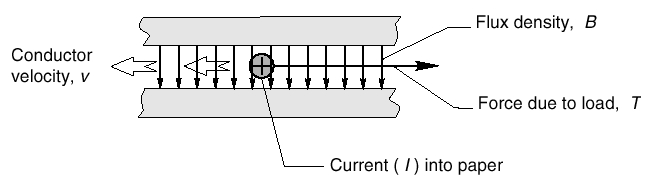
ill. 14 Diagrammatic sketch of primitive linear d.c. motor.
It is assumed that the conductor has a resistance (R), that it carries a d.c. current (I), and that it moves with a velocity (v) in a direction perpendicular to the field and the current (see ill. 14).Attached to the conductor is a string which passes over a pulley and supports a weight: the tension in the string acting as a mechanical 'load ' on the rod. Friction is assumed to be zero.
We need not worry about the many difficult practicalities of making such a machine, not least how we might manage to maintain electrical connections to a moving conductor. The important point is that although this is a hypothetical set-up, it represents what happens in a real motor, and it allows us to gain a clear understanding of how real machines behave before we come to grips with much more complex structures.
We begin by considering the electrical input power with the conductor stationary (i.e., v = 0). For the purpose of this discussion we can suppose that the magnetic field (B) is provided by permanent magnets. Once the field has been established (when the magnet was first magnetized and placed in position),no further energy will be needed to sustain the field, which is just as well since it's obvious that an inert magnet is incapable of continuously supplying energy. It follows that when we obtain mechanical output from this primitive 'motor ', none of the energy involved comes from the magnet. This is an extremely important point: the field system ,whether provided from permanent magnets or 'exciting ' windings, acts only as a catalyst in the energy conversion process, and contributes nothing to the mechanical output power.
When the conductor is held stationary the force produced on it (BIl) does no work, so there is no mechanical output power, and the only electrical input power required is that needed to drive the current through the conductor. The resistance of the conductor is R, the current through it's I, so the voltage which must be applied to the ends of the rod from an external source will be given by V_1 = IR, and the electrical input power will be V_1 I or I2 R .Under these conditions, all the electrical input power will appear as heat inside the conductor, and the power balance can be expressed by the equation
electrical input power (V_1 I ) = rate of production of heat in conductor (I2 R). (1.15)
Although no work is being done because there is no movement, the stationary condition can only be sustained if there is equilibrium of forces.
The tension in the string (T) must equal the gravitational force on the mass (mg), and this in turn must be balanced by the electromagnetic force on the conductor (BIl).Hence under stationary conditions the current must be given by
T = mg = BIl ,or I = mg/Bl (1.16)
This is our first indication of the link between the mechanical and electric worlds, because we see that in order to maintain the stationary condition, the current in the conductor is determined by the mass of the mechanical load. We will return to this link later.
Power relationships -- conductor moving at constant speed
Now let us imagine the situation where the conductor is moving at a constant velocity (v) in the direction of the electromagnetic force that's propelling it. What current must there be in the conductor, and what voltage will have to be applied across its ends? We start by recognizing that constant velocity of the conductor means that the mass (m)is moving upwards at a constant speed, i.e. it's not accelerating. Hence from Newton's law, there must be no resultant force acting on the mass, so the tension in the string (T) must equal the weight (mg).Similarly, the conductor isn't accelerating, so its net force must also be zero. The string is exerting a braking force (T), so the electromagnetic force (BIl) must be equal to T .Combining these conditions yields
T = mg = BIl ,or I = mg/Bl (1.17)
This is exactly the same equation that we obtained under stationary conditions, and it underlines the fact that the steady-state current is determined by the mechanical load. When we develop the equivalent circuit, we will have to get used to the idea that in the steady-state one of the electrical variables (the current) is determined by the mechanical load.
With the mass rising at a constant rate, mechanical work is being done because the potential energy of the mass is increasing. This work is coming from the moving conductor. The mechanical output power is equal to the rate of work, i.e. the force (T = BIl) times the velocity (v).
The power lost as heat in the conductor is the same as it was when stationary, since it has the same resistance, and the same current. The electrical input power supplied to the conductor must continue to furnish this heat loss, but in addition it must now supply the mechanical output power. As yet we don't know what voltage will have to be applied, so we will denote it by V 2.The power-balance equation now becomes
electrical input power (V2 I ) = rate of production of heat in conductor + mechanical output power = I2 R = (BIl)v (1.18)
We note that the first term on the right hand side of equation 1.18 represent the heating effect, which is the same as when the conductor was stationary, while the second term represents the additional power that must be supplied to provide the mechanical output. Since the current is the same but the input power is now greater, the new voltage V 2 must be higher than V 1.By subtracting equation 1.15 from equation 1.18 we obtain
V_2 I – V_1 I = (BIl)v
and thus
V_2 - V _1 = Blv = E (1.19)
Equation 1.19 quantifies the extra voltage to be provided by the source to keep the current constant when the conductor is moving. This in crease in source voltage is a reflection of the fact that whenever a conductor moves through a magnetic field, an EMF (E) is induced in it.
We see from equation 1.19 that the EMF is directly proportional to the flux density, to the velocity of the conductor relative to the flux, and to the active length of the conductor. The source voltage has to overcome this additional voltage in order to keep the same current flowing: if the source voltage isn't increased, the current would fall as soon as the conductor begins to move because of the opposing effect of the induced EMF
We have deduced that there must be an EMF caused by the motion, and have derived an expression for it by using the principle of the conservation of energy, but the result we have obtained, i.e.
E = Blv (1.20)
is often introduced as the 'flux-cutting 'form of Faraday 's law, which states that when a conductor moves through a magnetic field an EMF given by equation 1.20 is induced in it. Because motion is an essential part of this mechanism, the EMF induced is referred to as a 'motional EMF'. The 'flux-cutting 'terminology arises from attributing the origin of the EMF to the cutting or slicing of the lines of flux by the passage of the conductor. This is a useful mental picture, though it must not be pushed too far: the flux lines are after all merely inventions which we find helpful in coming to grips with magnetic matters.
Before turning to the equivalent circuit of the primitive motor, two general points are worth noting. Firstly, whenever energy is being converted from electrical to mechanical form, as here, the induced EMF always acts in opposition to the applied (source) voltage. This is reflected in the use of the term 'back EMF' to describe motional EMF in motors.
Secondly, although we have discussed a particular situation in which the conductor carries current, it's certainly not necessary for any current to be flowing in order to produce an EMF: all that's needed is relative motion between the conductor and the magnetic field.
EQUIVALENT CIRCUIT
We can represent the electrical relationships in the primitive machine in an equivalent circuit as shown in ill. 15.
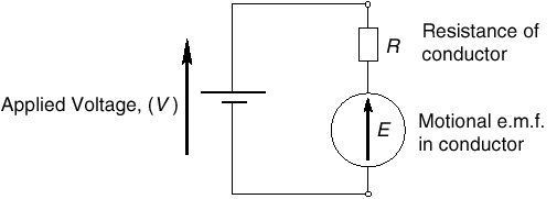
ill. 15 Equivalent circuit of primitive d.c. motor.
The resistance of the conductor and the motional EMF together represent in circuit terms what is happening in the conductor (though in reality the EMF and the resistance are distributed, not lumped as separate items).The externally applied source that drives the current is represented by the voltage V on the left (the old-fashioned battery symbol being deliberately used to differentiate the applied voltage V from the induced EMFE ).We note that the induced motional EMF is shown as opposing the applied voltage, which applies in the 'motoring 'condition we have been discussing. Applying Kirchoff's law we obtain the voltage equation as
V = E + IR or I = (V-E)/R (1.21)
Multiplying equation 1.21 by the current gives the power equation as electrical input power (VI) = mechanical output power (EI) + copper loss (I2 R). (1.22)
(Note that the term 'copper loss 'used in equation 1.22 refers to the heat generated by the current in the windings: all such losses in electric motors are referred to in this way, even when the conductors are made of aluminum or bronze!) It is worth seeing what can be learned from these equations because, as noted earlier, this simple elementary 'motor 'encapsulates all the essential features of real motors. Lessons which emerge at this stage will be invaluable later, when we look at the way actual motors behave.
If the EMF E is less than the applied voltage V, the current will be positive, and electrical power will flow from the source, resulting in motoring action. On the other hand if E is larger than V, the current will flow back to the source, and the conductor will be acting as a generator. This inherent ability to switch from motoring to generating without any interference by the user is an extremely desirable property of electromagnetic energy converters. Our primitive set-up is simply a machine which is equally at home acting as motor or generator.
A further important point to note is that the mechanical power (the first term on the right hand side of equation 1.22) is simply the motional EMF multiplied by the current. This result is again universally valid, and easily remembered. We may sometimes have to be a bit careful if the EMF and the current are not simple d.c. quantities, but the basic idea will always hold good.
Finally, it's obvious that in a motor we want as much as possible of the electrical input power to be converted to mechanical output power, and as little as possible to be converted to heat in the conductor. Since the output power is EI, and the heat loss is I2 R we see that ideally we want EI to be much greater than I2 R, or in other words E should be much greater than IR .In the equivalent circuit (ill. 15) this means that the majority of the applied voltage V is accounted for by the motional EMF (E), and only a little of the applied voltage is used in overcoming the resistance.
Motoring condition
Motoring implies that the conductor is moving in the same direction as the electromagnetic force (BIl),and at a speed such that the back EMF (Blu )is less than the applied voltage V .In the discussion so far, we have assumed that the load is constant, so that under steady-state conditions the current is the same at all speeds, the voltage being increased with speed to take account of the motional EMF This was a helpful approach to take in order to derive the steady-state power relationships, but is seldom typical of normal operation. We therefore turn to how the moving conductor will behave under conditions where the applied volt age V is constant, since this corresponds more closely with the normal operations of a real motor.
In the next section, matters are inevitably more complicated than we have seen so far because we include consideration of how the motor increases from one speed to another, as well as what happens under steady-state conditions. As in all areas of dynamics, study of the transient behavior of our primitive linear motor brings into play additional parameters such as the mass of the conductor (equivalent to the inertia of a real rotary motor)which are absent from steady-state considerations.
Behavior with no mechanical load
In this section we assume that the hanging weight has been removed, and that the only force on the conductor is its own electromagnetically generated one. Our primary interest will be in what determines the steady speed of the primitive motor, but we must begin by considering what happens when we first apply the voltage.
With the conductor stationary when the voltage V is applied, the current will immediately rise to a value of V/R, since there is no motional EMF and the only thing which limits the current is the resistance.
(Strictly we should allow for the effect of inductance in delaying the rise of current, but we choose to ignore it here in the interests of simplicity.)The resistance will be small, so the current will be large, and a high force will therefore be developed on the conductor. The conductor will therefore accelerate at a rate equal to the force on it divided by its mass.
ill. 16Dynamic (run-up) behavior of primitive d.c. motor with no mechanical load.
As it picks up speed, the motional EMF (equation 1.20) will grow in proportion to the speed. Since the motional EMF opposes the applied voltage, the current will fall (equation 1.21), so the force and hence the acceleration will reduce, though the speed will continue to rise. The speed will increase as long as there is an accelerating force, i.e. as long as there is current in the conductor. We can see from equation 1.21 that the current will finally fall to zero when the speed reaches a level at which the motional EMF is equal to the applied voltage. The speed and current therefore vary as shown in ill. 16: both curves have the exponential shape which characterizes the response of systems governed by a first-order differential equation. The fact that the steady-state current is zero is in line with our earlier observation that the mechanical load (in this case zero) determines the steady-state current.
We note that in this idealized situation (in which there is no load applied, and no friction forces), the conductor will continue to travel at a constant speed, because with no net force acting on it there is no acceleration. Of course, no mechanical power is being produced, since we have assumed that there is no opposing force on the conductor, and there is no input power because the current is zero. This hypothetical situation nevertheless corresponds closely to the so-called 'no-load ' condition in a motor, the only difference being that a motor will have some friction (and therefore it will draw a small current),whereas we have assumed no friction in order to simplify the discussion.
Although no power is required to keep the frictionless and unloaded conductor moving once it's up to speed, we should note that during the whole of the acceleration phase the applied voltage was constant and the input current fell progressively, so that the input power was large at first but tapered-off as the speed increased. During this run-up time energy was continually being supplied from the source: some of this energy is wasted as heat in the conductor, but much of it's stored as kinetic energy, and as we will see later, can be recovered.
An elegant self-regulating mechanism is evidently at work here. When the conductor is stationary, it has a high force acting on it, but this force tapers-off as the speed rises to its target value, which corresponds to the back EMF being equal to the applied voltage. Looking back at the expression for motional EMF (equation 1.18), we can obtain an expression for the no-load speed (v o) by equating the applied voltage and the back EMF, which gives
E = V = Blv_0, i.e :v_0 = V Bl (1.23)
Equation 1.23 shows that the steady-state no-load speed is directly proportional to the applied voltage, which indicates that speed control can be achieved by means of the applied voltage. We will see later that one of the main reasons why d.c. motors held sway in the speed-control arena for so long is that their speed could be controlled simply by controlling the applied voltage.
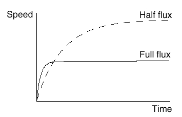
ill. 17 Effect of flux density on the acceleration and steady running speed of primitive d.c. motor with
no mechanical load.
Rather more surprisingly, equation 1.23 reveals that the speed is inversely proportional to the magnetic flux density, which means that the weaker the field, the higher the steady-state speed. This result can cause raised eyebrows, and with good reason. Surely, it's argued, since the force is produced by the action of the field, the conductor won't go as fast if the field was weaker. This view is wrong, but understandable.
The flaw in the argument is to equate force with speed. When the voltage is first applied, the force on the conductor certainly will be less if the field is weaker, and the initial acceleration will be lower. But in both cases the acceleration will continue until the current has fallen to zero, and this will only happen when the induced EMF has risen to equal the applied voltage. With a weaker field, the speed needed to generate this EMF will be higher than with a strong field: there is 'less flux ',so what there is has to be cut at a higher speed to generate a given EMF. The matter is summarized in ill. 17,which shows how the speed will rise for a given applied voltage, for 'full 'and 'half 'fields respectively. Note that the initial acceleration (i.e. the slope of the speed-time curve) in the half-flux case is half that of the full-flux case, but the final steady speed is twice as high. In real d.c. motors, the technique of reducing the flux density in order to increase speed is known as 'field weakening '.
Behavior with a mechanical load
Suppose that, with the primitive linear motor up to its no-load speed we suddenly attach the string carrying the weight, so that we now have a steady force (T = mg) opposing the motion of the conductor. At this stage there is no current in the conductor and thus the only force on it will be T .The conductor will therefore begin to decelerate. But as soon as the speed falls, the back Endwell become less than V ,and current will begin to flow into the conductor, producing an electromagnetic driving force. The more the speed drops, the bigger the current, and hence the larger the force developed by the conductor. When the force developed by the conductor becomes equal to the load (T), the deceleration will cease, and a new equilibrium condition will be reached. The speed will be lower than at no-load, and the conductor will now be producing continuous mechanical output power, i.e. acting as a motor.
Since the electromagnetic force on the conductor is directly proportional to the current, it follows that the steady-state current is directly proportional to the load which is applied, as we saw earlier. If we were to explore the transient behavior mathematically, we would find that the drop in speed followed the same first-order exponential response that we saw in the run-up period. Once again the self-regulating property is evident, in that when load is applied the speed drops just enough to allow sufficient current to flow to produce the force required to balance the load. We could hardly wish for anything better in terms of performance, yet the conductor does it without any external intervention on our part. Readers who are familiar with closed-loop control systems will probably recognize that the reason for this excellent performance is that the primitive motor possesses inherent negative speed feedback via the motional EMF. This matter is explored more fully later.
Returning to equation 1.21, we note that the current depends directly on the difference between V and E, and inversely on the resistance. Hence for a given resistance, the larger the load (and hence the steady-state current), the greater the required difference between V and E ,and hence the lower the steady running speed, as shown in ill. 18.
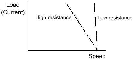
ill. 18 Influence of resistance on the ability
of the motor to maintain speed when load is applied. We can also see
from equation 1.21 that the higher the resistance of the conductor, the
more it slows down when a given load is applied.
Conversely, the lower the resistance, the more the conductor is able to hold its no-load speed in the face of applied load. This is also illustrated in ill. 18.We can deduce that the only way we could obtain an absolutely constant speed with this type of motor is for the resistance of the conductor to be zero, which is of course not possible. Nevertheless, real d.c. motors generally have resistances which are small, and their speed does not fall much when load is applied -a characteristic which for most applications is highly desirable.
We complete our exploration of the performance when loaded by asking how the flux density influences behavior. Recalling that the electromagnetic force is proportional to the flux density as well as the current, we can deduce that to develop a given force, the current required will be higher with a weak flux than with a strong one. Hence in view of the fact that there will always be an upper limit to the current which the conductor can safely carry, the maximum force which can be developed will vary in direct proportion to the flux density, with a weak flux leading to a low maximum force and vice-versa. This under lines the importance of operating with maximum flux density whenever possible.
We can also see another disadvantage of having a low flux density by noting that to achieve a given force, the drop in speed will be disproportionately high when we go to a lower flux density. We can see this by imagining that we want a particular force, and considering how we achieve it firstly with full flux, and secondly with half flux. With full flux, there will be a certain drop in speed which causes the motional EMF to fall enough to admit the required current. But with half the flux, for example, twice as much current will be needed to develop the same force. Hence the motional EMF must fall by twice as much as it did with full flux. However, since the flux density is now only half, the drop in speed will have to be four times as great as it was with full flux. The half-flux 'motor' therefore has a load characteristic with a load/speed gradient four times more droopy than the full-flux one. This is shown in ill. 19; the applied voltages having been adjusted so that in both cases the no-load speed is the same. The half-flux motor is clearly inferior in terms of its ability to hold the set speed when the load is applied.
We may be tempted to think that the higher speed which we can obtain by reducing the flux somehow makes for better performance, but we can now see that this isn't so. By halving the flux, for example, the no-load speed for a given voltage is doubled, but when the load is raised until rated current is flowing in the conductor, the force developed is only half, so the mechanical power is the same. We are in effect trading speed against force, and there is no suggestion of getting something for nothing.
Relative magnitudes of V and E, and efficiency
Invariably we want machines which have high efficiency. From equation 1.20, we see that to achieve high efficiency, the copper loss (I2 R) must be small compared with the mechanical power (EI), which means that the resistive volt-drop in the conductor (IR) must be small compared with either the induced EMF (E) or the applied voltage (V).In other words we want most of the applied voltage to be accounted for by the 'useful ' motional EMF, rather than the wasteful volt drop in the wire. Since the motional EMF is proportional to speed, and the resistive volt drop depends on the conductor resistance, we see that a good energy converter requires the conductor resistance to be as low as possible, and the speed to be as high as possible.
ill. 19Influence of flux on the drop in steady running speed when load is applied.
To provide a feel for the sort of numbers likely to be encountered, we can consider a conductor with resistance of 0.5 ohm ,carrying a current of 4A, and moving at a speed such that the motional EMF is 8 V. From equation 1.19, the supply voltage is given by
V = E + IR = 8 + (4 x 0.5) = 10 volts
Hence the electrical input power (VI) is 40 watts, the mechanical output power (EI) is 32 watts, and the copper loss (I2 R) is 8 watts, giving an efficiency of 80%.
If the supply voltage was doubled (i.e. V = 20 volts), however, and the resisting force is assumed to remain the same (so that the steady state current is still 4A), the motional EMF is given by equation 1.19 as
E = 20 (4 x 0.5) = 18 volts
which shows that the speed will have rather more than doubled, as expected. The electrical input power is now 80 watts ,the mechanical output power is 72 watts, and the copper loss is still 8 watts. The efficiency has now risen to 90%,underlining the fact that the energy conversion process gets better at higher speeds.
The ideal situation is clearly one where the term IR in equation 1.19 is negligible, so that the back EMF is equal to the applied voltage. We would then have an ideal machine with an efficiency of 100%, in which the steady-state speed would be directly proportional to the applied voltage and independent of the load.
In practice the extent to which we can approach the ideal situation discussed above depends on the size of the machine. Tiny motors, such as those used in wrist-watches, are awful, in that most of the applied voltage is used up in overcoming the resistance of the conductors, and the motional EMF is very small: these motors are much better at producing heat than they are at producing mechanical output power! Small machines, such as those used in hand tools, are a good deal better with the motional EMF accounting for perhaps 70 -80% of the applied voltage. Industrial machines are very much better: the largest ones (of many hundreds of kW) use only one or two percent of the applied voltage in overcoming resistance, and therefore have very high efficiencies.
Analysis of primitive motor -- conclusions
All of the lessons learned from looking at the primitive motor will find direct parallels in almost all of the motors we look at in the rest of this guide, so it's worth reminding ourselves of the key points.
Firstly, we will make frequent reference to the formula for the force (F) on a conductor in a magnetic field, i.e.
F = BIl (1.24)
and to the formula for the motional induced e.m.f, (E ) i.e.
E = Blv ( 1.25)
where B is the magnetic flux density, I is the current, l is the length of conductor and v is the velocity perpendicular to the field. These equations form the theoretical underpinning on which our understanding of motors will rest.
Secondly, we have seen that the speed at which the primitive motor runs unloaded is determined by the applied voltage, while the current that the motor draws is determined by the mechanical load Exactly the same results will hold when we examine real d.c. motors, and very similar relationships will also emerge when we look at the induction motor.