AMAZON multi-meters discounts AMAZON oscilloscope discounts
Sooner or later, every power supply designer finds out the hard way that if anything has the potential to cause a return to the drawing board at the very last moment, it's either a thermal issue, a safety related issue, or a stubborn EMI (electromagnetic interference) problem.
Of these, the first does get resolved relatively easily - more copper, better heatsinking, and hopefully more air. The safety issues also melt away, with a little prescience during the design phase - and later by some heat shrink tubing, tie-wraps, liberally applied hot-melt glue, RTV (room temperature vulcanizing - i.e. silicone glue), and so on. But we discover that EMI turns out to be a veritable "balloon" - if we try to "push" in the emissions spectrum on one side, it "bulges" out at the other. We manage to achieve compliance with regulatory conducted emission limits, only to find it has been at the expense of the radiated limits, or vice versa. And sadly, our trusted little bag of tricks (and that dusty Fair-Rite kit of beads) may also sometimes mysteriously let us down. It's then we realize rather acutely - if we can't comply, we can't sell! The stumbling block to a successful understanding of this very vital but misunderstood area of power conversion is that some of the terminology and descriptions used by signal integrity engineers to describe EMI have been bandied about a little too freely in power. Sure there are great similarities, but the devil is in the details. Maybe that's why all the EMI FAQs and 'EMI for Dummies' help-books just didn't seem to help. This general feeling of helplessness has ultimately translated into a popular perception that there is some black magic involved in EMI. Actually, as we will see, all that's really needed is some high school physics, some simple math, and a clear conceptual understanding for all things "power." That said, EMI is admittedly a challenging area, partly because a lot of uncharacterized parasitics enter the stage, each vying for attention. So bench tweaking isn't going to be completely avoidable. But with a clear insight into EMI, any major redesign should never be required. It is plain however, that for this to happen, the engineer just can't afford to wait until the penultimate moments of the project before he or she takes EMI seriously. It is important to get in early, and get in close - with a clear insight into EMI as applied to power conversion. The alternative is the high cost involved in waiting, redesigning, and also days of fruitless and expensive test lab time.
- EME = Electromagnetic Emission
- EMS = Electromagnetic Immunity/Susceptibility
- CE = Conducted Emission
- CS = Susceptibility to Conducted Emissions
- RE = Radiated Emission
- RS = Susceptibility to Radiated Emissions
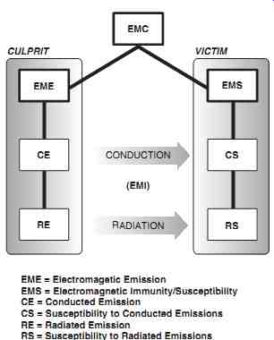
Fgr 1:
The EMI/EMC "Tree" (emissions and susceptibility)
The Standards
The issues of safety and 'electromagnetic compliance' (EMC) are usually clubbed together in most countries. The CE mark (i.e. European Conformity mark) is one such example. Another is the CCC mark (China Compulsory Certification - required by the People's Republic of China, i.e. mainland China). Generally speaking, designated product categories must carry such marks in their respective market regions, and are then assumed to comply with both the valid safety and EMC standards. In the United States, though, the issues of safety and EMC are taken up separately. The "UL mark" (Underwriters Laboratory Inc.) indicates compliance to product safety standards, whereas "FCC certification" (Federal Communications Commission) reflects compliance with electromagnetic interference (EMI) standards. But EMI is only one note in the gamut of EMC (see Fgr 1). In the United States, unlike Europe, the 'susceptibility' aspect of EMC has been left to the dictate of market forces rather than to the force of law. In Japan, the situation is that though EMC specifications exist, they are stated specifically only for IT (information technology) equipment (or 'ITE'). In addition, the decision to actually affix the relevant mark (called the VCCI label, for Voluntary Control Council for Interference) is completely voluntary (as the name itself suggests). But we must realize that all such EMI/EMC/Safety marks, whether required by regional/national laws or not, are increasingly perceived by the market as an indication of product quality. Thus, though in theory some of these may be voluntary, in practice, marketing pressures may make them inevitable.
How deep should the power supply engineer really delve into the details of standards and regulations? The road is undoubtedly tricky, because the standards themselves are in a state of continuous evolution. And even though the underlying intent is the same, the various international standards can appear quite diverse. Even where supposedly uniform standards have been accepted, there may be national or regional 'deviations.' And even if, hypothetically speaking, the standards were all identical (and there is a definite movement toward that), the certification aspects are never likely to be identical in all countries. The bottom line is that no relevant information that can be provided here, or elsewhere, will turn out to be durable enough to withstand the scrutiny of time. So a timely chat with a recognized test lab or consultant should, in any case, always be on a developmental checklist. With that reassurance in mind, the engineer will probably best spend his or her time mastering the engineering aspects of EMI/EMC, that being something about which that test house can't really provide detailed guidance.
But the engineer still needs to know how far he or she needs to go down the engineering route to achieve necessary compliance - and hopefully, as easily and cost-effectively as possible. The good news here is that, as mentioned, despite the present diversity in regulations, there exists a clear and steady movement toward a set of universally accepted (harmonized) standards. The EMI/EMC standards in all the countries and regions mentioned previously, and in fact in most others around the world, are increasingly based on (if not identical to) a well-known set of European standards. Note that, previously accepted norms or standards that were recognizable by familiar prefixes - 'VDE,' 'CISPR,' 'IEC,' and 'ISO,' have all been steadily converging into a single set of pan-European norms prefixed 'EN.' A typical power supply engineer is therefore almost always concerned about just achieving compliance with the European EMI standard called "EN 550022" (meant for IT equipment). This standard was originally (and in fact popularly even now) known as CISPR 22. It is the standard we too will be largely focusing on. The corresponding U.S. standard is "FCC Part 15." Despite some differences, the FCC accepts testing to CISPR 22 standards. In fact in 2002, the FCC harmonized Part 15 completely to CISPR 22, laying out a transition period for manufacturers to eventually comply.
As an example of how other countries tend to follow the lead set by Europe and the United States in these matters, take Canada for example. The regulatory Canadian body having jurisdiction over EMI is called 'Industry Canada.' However, its technical requirements are essentially equivalent to those of the FCC. Therefore, if FCC approval has been obtained (either by meeting Part 15 of the FCC rules or CISPR 22), the equipment need not be retested.
Maxwell to EMI
Light, radio-frequency waves, infrared radiation, microwaves, and so on are all electromagnetic waves (see Fgr 2). For all these, the basic relationship connecting their wavelength λ (in m), their frequency f (in Hz), and the speed of the wave u in the medium of propagation (in m/s), is given by λ = u/f . For a wave propagating in free space (or air), the speed u is called 'c' and has the value 3 × 10⁸ m/s. An easy form to remember is λ _meters = 300 f_MHz The ratio c/u is always greater than 1, and is called the index of refraction of the material (through which the wave travels at the speed u). Note that though c is popularly called the velocity of light, it's the same for any electromagnetic wave. It can be shown that c = 1/SQR-RT(µoeo), where µo is the permeability of free space (vacuum or air) and eo is the permittivity of free space. µo and eo are fundamental constants, since they represent the properties of our universe.
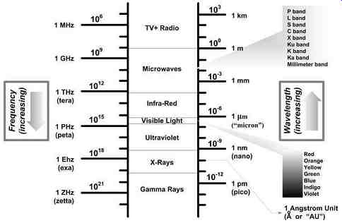
Fgr 2: The Electromagnetic Environment
It is well-known from our physics class that if a piece of electronic equipment has a dimension close to λ/4, it can end up radiating (or receiving) the corresponding frequency very effectively. This is the principle behind a radio antenna. Note that although a TV antenna is symmetrical around the point where it connects to the cable and has a total physical length of λ/2, it actually has only λ /4 (effective receiving length) on each side.
But what if an antenna is much shorter than the 'optimum' of λ /4? Antennas are actually quite effective down to less than λ/10 - which explains why we can pick up almost all the FM stations well enough from a (fixed length) whip antenna on our car. But what if the antenna is much longer than λ /4? In that case, we can consider the antenna as, in effect, being clamped at λ /4 - the remaining length basically superfluous. Therefore, we should never judge an antenna by its length! When we plug a piece of equipment to the ac power lines, its input cable (ac line cord) can combine with the wiring of the building to form an antenna. This can produce strong radiated interference that can affect the operation of other devices in the vicinity. In addition to the radiation process, the emissions can also just conduct through the mains wiring, and thereby directly affect other similarly plugged-in devices. Therefore, there are distinct radiated emission limits and conducted emission limits specified within all EMI regulatory standards.
We have realized that it would be a mistake to jump to the conclusion that a certain cable length or PCB (printed circuit board) trace is either "too short" or "too long," and therefore not contributing to a certain stubborn EMI peak we may be observing. Further, we should keep in mind that any antenna is as good a receiver, as it's a transmitter. So we could have a situation where radiation is originally generated by the output cables, but then picked up by the input cables (by radiation), from which point onward it gets conducted into the wiring of the building (or/and radiated once again). In fact, we will find that the input and output cables are often responsible for a lot of high-frequency EMI noise, both in the radiated spectrum and the conducted spectrum.
Concerns about cable length take on a whole new meaning when they are coupled with circuits containing modern high-speed digital chips. Such chips are themselves powerful EMI emitters, but with the help of inadvertent antennas like the surrounding PCB traces and cables, and also with the inadvertent help of various board, component, and enclosure parasitics, they can put on quite a show! Courtesy Maxwell! Maxwell showed that whenever an electric field (the 'E-field'- dimensions V/m) varies with time, it produces a magnetic field (the 'H-field'- dimensions A/m), and vice versa.
In fact, the better-known Faraday's law of induction (without which no transformer in the world would exist) is actually the first of the set of four Maxwell's unifying equations. So we learn that the E- and H-fields appear simultaneously, the moment the original magnetic or electric source has a time variance. At some distance away, these fields combine to form an electromagnetic wave - that propagates out into space (at the speed of light).
We know that any capacitor that's charged up has an associated E-field residing in the space between the plates, and thus a "resident energy" term of (1/2) × CV2. We certainly don't expect to have any associated H-field, simply because there is no current flowing once everything is "steady" (ignoring leakage current). However during the capacitor charging process (as the capacitor voltage is rising from zero to its final value), there is a charging current passing through the capacitor. So during that time, both E- and H-fields are generated. Applying the same analogy to a coil passing a steady dc current - it has an associated H-field, with a resident energy of (1/2)LI 2 in 'steady state'- but no E-field.
Note that in power supplies, there are various subtle connotations to the word 'steady state.' But in the sense used above, a power supply is really not "steady" - except perhaps in its steady repetitiveness. In other words, in every switching cycle, the inductor current is actually ramping up and then down, between two extremes. So this pattern is certainly steady, but the currents and voltages aren't, since they are constantly changing. So, as the current undulates, there is a constantly changing H-field and an accompanying E-field.
Together, these two fields constitute an electromagnetic field in the vicinity of the coil (forming an electromagnetic wave only a certain distance away). That is why, in switching power converters, EMI has become such a major concern. E.g., rod inductors (often used in post-LC filters at the output) are nicknamed 'EMI cannons' by some engineers. They spew energy all around, and special precautions are needed to prevent this energy from conducting or radiating over to greater distances.
We can ask - what really makes modern digital chips and modern switching converters worse from the standpoint of EMI? That is because of the escalating frequencies involved.
Smaller and smaller PCB traces and lead lengths can become effective antenna at very high frequencies. So nowadays we are getting painfully aware of the fact that as the frequency increases, so can the intensity of these fields (at a certain distance). Note however, that when talking about switching power converters, the "frequency" that we are talking about isn't necessarily the basic PWM switching frequency (which is only of the order of say 100-500 kHz - i.e. a time period of a few microseconds). We are referring more to the exceedingly fast transition times - which are of the order of 10 to 100 ns only. The Fourier analysis of such a switching waveform will reveal a large amount of very high-frequency content, associated with the actual switch transitions. These can cause far more EMI.
Maxwell's equations are usually written out in a way that doesn't fully reveal the following fact very clearly - it turns out that it really does not matter whether we are talking about waveforms of switched voltages (time varying E-fields) or of switched currents (time varying H-fields) - eventually their respective equations are complementary and are thus very similar. Further, these two fields become proportional to each other at a large distance away, constituting an electromagnetic wave, one that can travel great distances on its own.
It also follows that if we can 'kill' one component of an electromagnetic wave (either its E-field or H-field), we will manage to kill the entire wave.
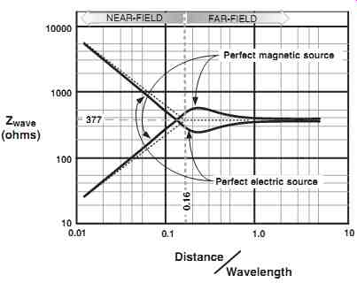
Fgr 3: Impedances in Free Space
If we consider the ratio of the amplitudes of E and H of an electromagnetic wave, we will see that though these fields decrease as the distance from the source increases, their ratio remains constant at any point sufficiently far away. The proportionality constant depends on the material of propagation, being equal to E/H = SQR-RT(µ_o/e_o), where µ is the permeability of the material (of propagation), and e its permittivity. Note that e is the electrical analog of the magnetic parameter µ that describes the extent to which a given material allows itself to become magnetized by an external magnetic field. We also note that the units of E are V/m, and H is A/m. Therefore the ratio E/H has the units V/A which is simply a resistance (ohms).
In air or vacuum (free space), E/H = SQR-RT(µ_o/e_o) = 120 · pi = 377 ohms. The subscript 'o,' used for the permeability and permittivity above, now refers to free space.
If the fields are very close to the source (as compared to the wavelength of their associated EMI wave), they don't follow the simple rules described above. See Fgr 3 for example, for the possible range of impedances for these so-called 'near-fields.' (Near-fields are defined as those at distances less than λ/6 from the source.) It also becomes clear why it's often colloquially said that "E-fields have high impedance," whereas "magnetic fields have low impedance." A small circular current loop of trace on a PCB produces magnetic fields, but a strip of copper or metal with a swinging voltage on it (e.g. a heatsink) forms a source of electric fields. Of course, once there is time-variance involved, the H-field leads to an associated E-field, and an E-field produces H-fields. However, only at a great distance away do the E- and H-fields become proportional to each other and thus form an electromagnetic wave.
As a real-life example of how apparently small-sized circuits can cause major EMI problems, consider a circular current loop (diameter « wavelength) enclosing an area "A" (m2) carrying an ac current of amplitude "I" (in amperes) and of frequency "f" (in Hz). Its field pattern can be broken up into a near-field (x < λ/2p) and a far-field (x > λ/2p). The far-field (the electromagnetic wave) at a distance x from the center of the coil, when calculated in the plane containing the loop, can be shown to be:
H =[ pi · I · A/λ2 - x ] A/m
… where E/H = 377 ohms is called the wave impedance in free space, or the intrinsic impedance of free space. We can see that as wavelength decreases (frequency increases), the field strength increases. Note that (for far-fields) both E and H vary as the reciprocal of the distance. But if we get closer and closer to an electric or magnetic source, we could ultimately find field components varying as 1/x, 1/x2, and 1/x^3. But more importantly, we will also see that the dependence on distance of the E-field is no longer the same as that of the H-field. Therefore their ratio too now keeps changing as the distance decreases. They are therefore said to constitute an (local) electromagnetic field (not a wave).
In standard radiated EMI tests, the specified measurement range of frequencies is 30 MHz and above (usually up to 1 GHz). An antenna is placed to sense the fields at a specified distance from the device. FCC specifies this distance to be 3 m, whereas CISPR requires 10 m. Let us see why there is actually no conflict here (usually).
The distance from the source that corresponds to the boundary between what is considered a near-field and what is a far-field is given by:
π / 2p = c/f x l/2 π = 1.6 m
Note that λ/2p = 0.16m, as was used in Fgr 3. A simpler way to remember the above relationship is as follows - if we call the boundary between the near- and far-field 'X' (expressed in meters), the corresponding frequency (in MHz) is:
f_MHz = 48/X_meters
So a measurement distance of 3 m can be considered a "near-field" distance only for frequencies of 48/3 = 16 MHz and below. But that's well below the range of frequencies of interest for a typical radiated EMI test (30 MHz to 1 GHz). Therefore we can conclude that over the specified test frequency range, we will only see far-fields.
Coming to CISPR, only frequencies lower than 4.8 MHz can present near-fields at the specified distance of 10 m. That is even further below the range of concern in a radiated test. Therefore, knowing that the measured field is a far-field for either of the two standards, we can then deduce that the radiated emissions level must be varying with distance as 1/x. That makes it finally possible to compare apples to apples. Therefore, the 3 m FCC reading can be easily scaled to a 10 m CISPR reading (and vice versa). The reading at 3 m (FCC) as compared to a reading at 10 m (CISPR) will differ by:
20 × log E3m/E10m = 20 × log 10/3 = 10.5 dB
So if we add 10.5 dB to any radiation spectrum measured as per CISPR, we get the equivalent FCC spectrum. This variation is referred to in the standards as an "inverse linear distance extrapolation factor of 20 dB per decade." Note that we are talking of a decade of distance, not of frequency or amplitude! And 20 dB per decade of distance is simply another way of stating a 1/x dependency (1/x2 would be 40 dB/decade). So for example, a 1/x (far) field at 30 m would be related to the field at 3 m by:
20 × log E3m/E30m = 20 × log 30/3 = 20 dB
CISPR 22 also says that if the ambient noise levels are too high at 10 m, we can do the measurement at 3 m, and basically add 10.5 dB uniformly to the 10 m limits.
We also note that radiated tests usually only bother to measure the E-field - since the H-field is then automatically known, being proportional to the E-field. Of course, the near-field and far-field definitions assume a point source. Therefore, especially in the case of the 3 m test, some further validation to prove that we really do have only far-fields may become necessary.
Susceptibility/Immunity
Looking at Fgr 1 again, we realize that it can also happen that when interference from the culprit does affect the operation of a device in the vicinity (the victim), it may simply be because the victim device is overly sensitive to EMI. Therefore to assure a prospective buyer that his equipment or device isn't going to malfunction whenever someone in the adjacent building just turns on an electric shaver or vacuum cleaner, for example, governments recommend (as in the United States) or mandate (as in the European Union) that a certain tolerance to incoming EMI be built into the device -- or at least be specified clearly for the customer to know beforehand. Now, since all rules must apply equally to all equipment big or small, including the culprit itself in this case, it follows that any equipment shouldn't emit too much EMI or be too susceptible to it. These issues are thus two sides of the same coin, and are therefore considered central to the concept of electromagnetic compatibility (EMC).
Electromagnetic compatibility (EMC) is therefore defined as the ability of equipment or systems to share the electromagnetic environment (much like we share our freeways).
Devices should operate satisfactorily, without either inducing (emitting) or experiencing interference from others. Note that the sensitivity of a device to electromagnetic fields is alternatively described as its immunity rather than its susceptibility.
Recognizing that the local environment plays a role in defining the amount of received interference and its acceptability, EMI limits are split into two basic application categories:
++ Class A, corresponding to commercial/industrial equipment/environment
++ Class B, corresponding to domestic or residential equipment Clearly, Class B limits will be more restrictive. In fact, these are roughly about 10 dB lower than Class A limits. That is a ratio of about 1:3 in terms of the actual amplitudes of the emission levels.
Like Class A and Class B emission limits, there are also different levels of immunity too.
The manufacturer usually specifies the level of tolerance his or her equipment is designed to meet. Based on certain specified test disturbance signals, the generic levels of susceptibility/ immunity are:
++ Type A: Performance during the test does not fall below a level set by the manufacturer (usually the normal operating level of performance).
++ Type B: Though performance degradation is possible during the test, normal performance returns automatically after the test ceases, and with no loss of stored data or any change in the operational characteristics.
++ Type C: Restoration of normal performance after the test requires operator intervention (not skilled personnel) and the use of normally accessible controls (like a reset toggle switch on the outside).
++ Type D: Non-recovering failure (possible permanent damage). Includes anything that does not fall within the three types of immunity levels listed above.
Note: There are some situations where the interpretation of the law may not be very clear-cut. We may therefore also get as many opinions as the number of consultants we talk to! E.g. what if the proposed equipment is meant for an industrial installation, but the same electric utility lines are providing power to a nearby residential area? Should we comply with Class A or Class B? Generally speaking, in such cases, to avoid last minute delays and a possible redesign, we should err on the side of caution. In this case that means we should design to Class B limits at the very outset.
Some Cost-related Rules-of-thumb
A brief look at possible costs:
++ The FCC spectrum for digital equipment (currently) begins at 450 kHz, while the equivalent CISPR/EN regulations start at 150 kHz. So FCC compliance can be achieved with a relatively small and inexpensive filter.
++ CISPR/EN Class A compliance often requires a filter with at least twice the volume of the FCC-level unit. This filter can therefore be up to 50% more expensive.
++ CISPR/EN Class B compliance can require a filter with three to ten times the volume of the FCC unit, and could cost up to 4 times more.
Note: CISPR limits apply to line voltages of 230 VAC, whereas FCC limits are tested at United States line voltage (115 VAC). For a given output power, the input operating current is higher if the input voltage is less. Therefore, in any equipment designed to operate at United States line voltages, thicker copper is required in the filter chokes, and that's somewhat of a cost adder.
EMI for Subassemblies EMC is generally considered a system-level concern, since from the legal perspective, it applies only to the end-equipment. So a component power supply (also called an 'OEM' power supply or a 'subassembly,' e.g. the one inside our desktop computer) does not usually have to meet any EMI/EMC standard per se, unlike a stand-alone power supply. So the ultimate EMC responsibility rests with the system manufacturer. However, take the case of a component off-line power supply (a front-end converter) for example. Here, a major component of the EMI at the input of the system will clearly be coming from the power supply. So it certainly won't help if the power supply itself is producing more EMI than the limits that would apply to the overall system. We should also remember that when the power supply is integrated with the equipment, there are always some hard-to-predict interactions between the power supply and the rest of the system - through the connectors, wiring, chassis, grounding, and so on. So the final EMI isn't necessarily just the arithmetic sum (in dB) of the different subassemblies. Keeping this in mind, the system manufacturer would most likely call out for a front-end converter to maintain its EMI to less than 6 to 10 dB below the legal limits. That would usually leave enough headroom for the rest of his circuitry, and also for unexpected interactions. In addition, certification labs themselves may require the submitted prototypes be at least 2 to 3 dB below certification limits - so as to leave a margin for variations in subsequent production. Summing all this up - the practical resulting situation for front-end OEM converters is simply this -- yes, they don't need to comply with the legal EMI limits, in fact they need to be much better! What about dc-dc converters that happen to be positioned deep inside the equipment? Again, there are no legally valid EMI/EMC standards for these. Further, since they are likely to be preceded by various circuits and filters, surge suppressors, fuses, capacitors, inrush limiters, and so on (e.g. in the front-end power supply), there is usually an adequate (and fortuitous) EMI barrier already present, that prevents noise from the dc-dc converter from getting on to the ac mains lines via conduction. So, assuming an effective EMI radiation shield is also present (e.g. the grounded metal enclosure), radiated interference may also not be of great concern. Therefore typically, for low-power on-board dc-dc converters, no dedicated input filter stages may be required. However, if such a filter becomes necessary, it can usually just be a simple single-stage LC circuit - possibly even using a small ferrite bead inductor for the L of the filter. And sometimes, just one such filter stage may be good enough to service several paralleled converters.
Nowadays, manufacturers of dc-dc converter modules are often going through the trouble of profiling the EMI spectrum present at the (unfiltered) inputs of their products. The purpose is that, whether it's legally required or not, the information will certainly come in handy to the system designer when he or she makes EMI-related decisions. But often, even the outputs of modules are being EMI-profiled nowadays. The question arises -- why do we even need to test the outputs (for EMI)? In fact, old-school power supply designers are somehow reflexively conditioned into accepting the concept of noise at the input cables, since they visualize the input rails as being rather coarsely regulated, and thus with lots of ripple. They also tend to think that the output voltage rails are relatively 'smooth' since they carry regulated "dc," and can therefore be considered "quiet." But in reality, even the outputs can send forth significant amounts of high-frequency noise, which can often turn out to be even more stubborn than the relatively lower frequency EMI components present at the input.
Further, like the input, the output rails from the module or power supply may also be looking into long cable runs (as in telecom applications and distributed power networks). This we know will create a wide-band antenna for EMI. And, as mentioned earlier, the output radiation can be picked up by the input cables, aggravating the problem at the input too.
CISPR 22 for Telecom Ports-Proposed Changes
There is an ongoing debate about extending CISPR 22 to include mandatory full testing on telecom ports. Telecommunication ports are defined as those "which are intended to be connected to telecommunications networks (e.g. public-switched telecommunications networks, integrated services digital networks), local-area networks (e.g. Ethernet, Token Ring), and similar networks." There is also a possibility that other product standards will also start referencing these tests for signal lines in general. The new regulations came into effect in 2001, then again in 2003, but have been successively delayed.
One stumbling block has been that the contemplated test would require a special "ISN" (Impedance Stabilizing Network) -- which was apparently in short supply. Note that a more readily available ISN, called the 'LISN' (Line Impedance Stabilizing Network), is commonly used to test the inputs of an off-line power supply. It works by placing an impedance of 50 ohm between each input line and earth ground -- so as to closely simulate typical mains wiring impedances. But the proposed telecom ISN would require the impedance to be raised to 150 ohm -- that figure being more representative of the actual impedances occurring on typical data networks.
It is increasingly clear that eventually, the law is going to place significant additional EMI requirements on all on-board power converters and any power supply, off-line or otherwise, working inside telecom equipment. Therefore, in the not so unforeseeable future, we could soon all be routinely testing the outputs of every power supply in much the same manner as we test their inputs today. In fact even as of now, many of the big telecom equipment manufacturers, of their own volition, routinely comply with CISPR 22 limits on both the inputs and outputs of their telecom power supplies. Of course, instead of the special proposed ISN, they have just gone ahead and used the more readily available input LISN to test the outputs too.
Also see: Electromagnetic Interference (EMI) in Switching-Mode Power Supplies; Faraday Screens