AMAZON multi-meters discounts AMAZON oscilloscope discounts
5. Geological Risk Factors and Geo-Electric Field Response
Considerable prior work has been done to model the geomagnetic induction effects in ground-based systems. As an extension to this fundamental work, numerical modeling of ground conductivity conditions have been demonstrated to provide accurate replication of observed geo-electric field conditions over a very broad frequency spectrum. Past experience has indicated that 1D earth conductivity models are sufficient to compute the local electric fields. Lateral heterogeneity of ground conductivity conditions can be significant over meso-scale distances. In these cases, multiple 1D models can be used in cases where the conductivity variations are sufficiently large.
Ground conductivity models need to accurately reproduce geo-electric field variations that are caused by the considerable frequency ranges of geomagnetic disturbance events from the large- magnitude/ low-frequency electrojet-driven disturbances to the low-amplitude but relatively high-frequency impulsive disturbances commonly associated with magnetospheric shock events. This variation of electro magnetic disturbances therefore require models accurate over a frequency range from 0.3 to as low as 0.00001 Hz. At these low frequencies of the disturbance environments, diffusion aspects of ground conductivities must be considered to appropriate depths. Therefore, skin depth theory can be used in the frequency domain to determine the range of depths that are of importance. For constant earth conductivities, the depths required are more than several hundred kilometers, although the exact depth is a function of the layers of conductivities present at a specific location of interest.
It is generally understood that the earth's mantle conductivity increases with depth. In most locations, ground conductivity laterally varies substantially at the surface over mesoscale distances; these conductivity variations with depth can range from 3 to 5 orders of magnitude. While surface conductivity can exhibit considerable lateral heterogeneity, conductivity at depth is more uniform, with conductivities ranging from values of 0.1 to 10 S/m at depths from 600 to 1000 km. If sufficient low-frequency measurements are avail able to characterize ground conductivity profiles, models of ground conductivity can be successfully applied over mesoscale distances and can be accurately represented by use of layered conductivity profiles or models.
For illustration of the importance of ground models on the response of geo-electric fields, a set of four example ground models have been developed that illustrate the probable lower to upper quartile response characteristics of most known ground conditions, considering there is a high degree of uncertainty in the plausible diversity of upper layer conductivities. FIG. 7 provides a plot of the layered ground conductivity conditions for these four ground models to depths of 700 km. As shown, there can be as much as four orders of magnitude variation in ground resistivity at various depths in the upper layers. Models A and B have very thin surface layers of relatively low resistivity. Models A and C are characterized by levels of relatively high resistivity until reaching depths exceeding 400 km, while models B and D have high variability of resistivity in only the upper 50-200 km of depth.
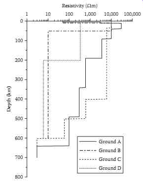
FIG. 7 Resistivity profiles versus depth of four examples of the layered
earth ground models.
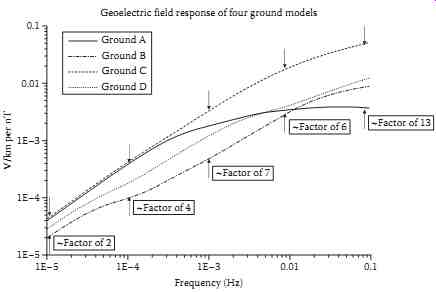
FIG. 8 Frequency response of four examples of the ground models of
FIG. 7; max/min geo-electric field response characteristics shown at
various discrete frequencies.
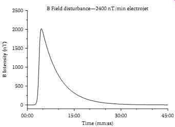
FIG. 9 Waveform of an electrojet-driven geomagnetic field disturbance
with 2400 nT/min rate of change intensity.
FIG. 8 provides the frequency response characteristics for these same four-layered earth ground models of FIG. 7. Each line plot represents the geo-electric field response for a corresponding incident magnetic field disturbance at each frequency. While each ground model has unique response characteristics at each frequency, in general, all ground models produce higher geo-electric field responses as the frequency of the incident disturbance increases. Also shown on this plot are the relative differences in geo-electric field response for the lowest and highest responding ground model at each decade of frequency. This illustrates that the response between the lowest and highest responding ground model can vary at discrete frequencies by more than a factor of 10. Also because the frequency content of an impulsive disturbance event can have higher frequency content (for instance due to a shock), the disturbance is acting upon the more responsive portion of the frequency range of the ground models. Therefore, the same disturbance energy input at these higher frequencies produces a proportionately larger response in geo-electric field. For example, in most of the ground models, the geo-electric field response is a factor of 50 higher at 0.1 Hz compared to the response at 0.0001 Hz.
From the frequency response plots of the ground models as provided in FIG. 8, some of the expected geo-electric field response due to geomagnetic field characteristics can be inferred. For example, Ground C provides the highest geo-electric field response across the entire spectral range, therefore, it would be expected that the time-domain response of the geo-electric field would be the highest for nearly all B field disturbances. At low frequencies, Ground B has the lowest geo-electric field response while at frequencies above 0.02 Hz, Ground A produces the lowest geo-electric field response. Because each of these ground models have both frequency-dependent and nonlinear variations in response, the resulting form of the geo-electric field waveforms would be expected to differ in form for the same B field input disturbance. In all cases, each of the ground models produces higher relative increasing geo-electric field response as the frequency of the incident B field disturbance increases. Therefore it should be expected that a higher peak geo-electric field should result for a higher spectral content disturbance condition.
A large electrojet-driven disturbance is capable of producing an impulsive disturbance as shown in FIG. 9, which reaches a peak delta B magnitude of ~2000 nT with a rate of change (dB/dt) of 2400 nT/min. This disturbance scenario can be used to simulate the estimated geo-electric field response of the four example ground models. FIG. 10 provides the geo-electric field responses for each of the four ground models for this 2400 nT/min B field disturbance. As expected, the Ground C model produces the largest geo-electric field reaching a peak of ~15 V/km, while Ground A is next largest and the Ground B model produces the smallest geo-electric field response. The Ground C geo-electric field peak is more than six times larger than the peak geo-electric field for the Ground B model. It is also evident that significant differences result in the overall shape and form of the geo-electric field response.
For example, the peak geo-electric field for the Ground A model occurs 17 s later than the time of the peak geo-electric field for the Ground B model. In addition to the differences in the time of peak, the waveforms also exhibit differences in decay rates. As is implied from this example, both the magnitudes of the geo-electric field responses and the relative differences in responses between models will change dependent on the source disturbance characteristics.
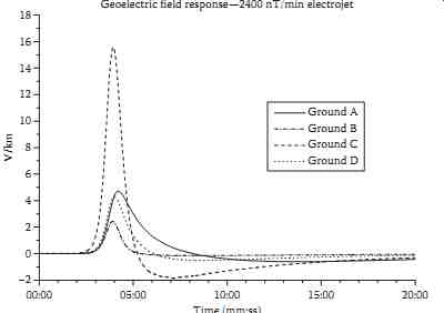
FIG. 10 Geo-electric field response of the four examples of ground
models to the 2400 nT/min disturbance conditions of FIG. 9.
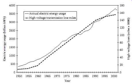
FIG. 11 Growth of the high-voltage transmission network and annual
electric energy usage in the United States over the past 50 years. In
addition to increasing the total network size, the network has grown
in complexity with the introduction of higher kV-rated lines that tend
to carry larger GIC flows.
6. Power Grid Design and Network Topology Risk Factors
While the previous discussion on ground conductivity conditions are important in determining the geo-electric field response, and in determining levels of GICs and their resulting impacts, power grid design is also an important factor in the vulnerability of these critical infrastructures, a factor in particular that over time has greatly escalated the effective levels of GIC and operational impacts due to these increased GIC flows. Unfortunately, most research into space weather impacts on technology systems has focused upon the dynamics of the space environment. The role of the design and operation of the technology system in introducing or enhancing vulnerabilities to space weather is often overlooked. In the case of electric power grids, both the manner in which systems are operated and the accumulated design decisions engineered into present-day networks around the world have tended to significantly enhance geomagnetic storm impacts. The result is to increase the vulnerability of this critical infra structure to space weather disturbances.
Both growth of the power grid infrastructure and design of its key elements have acted to introduce space weather vulnerabilities. The U.S. high-voltage transmission grid and electric energy usage have grown dramatically over the last 50 years in unison with increasing electricity demands of society. The high-voltage transmission grid, which is the part of the power network that spans long distances, couples almost like an antenna through multiple ground points to the geo-electric field produced by disturbances in the geomagnetic field. From Solar Cycle 19 in the late 1950s through Solar Cycle 22 in the early 1980s, the high-voltage transmission grid and annual energy usage have grown nearly tenfold ( FIG. 11).
In short, the antenna that is sensitive to space weather disturbances is now very large. Similar development rates of transmission infrastructure have occurred simultaneously in other developed regions of the world.
As this network has grown in size, it has also grown in complexity and sets in place a compounding of risks that are posed to the power grid infrastructures for GIC events. Some of the more important changes in technology base that can increase impacts from GIC events include higher design voltages, changes in transformer design, and other related apparatus. The operating levels of high-voltage networks have increased from the 100-200 kV thresholds of the 1950s to 400-765 kV levels of present-day networks.
With this increase in operating voltages, the average per unit length circuit resistance has decreased while the average length of the grid circuit increases. In addition, power grids are designed to be tightly interconnected networks, which present a complex circuit that is continental in size. These interrelated design factors have acted to substantially increase the levels of GIC that are possible in modern power networks.
In addition to circuit topology, GIC levels are determined by the size and the resistive impedance of the power grid circuit itself when coupled with the level of geo-electric field that results from the geo magnetic disturbance event. Given a geo-electric field imposed over the extent of a power grid, a current will be produced entering the neutral ground point at one location and exiting through other ground points elsewhere in the network. This can be best illustrated by examining the typical range of resistance per unit length for each kV class of transmission lines and transformers.
As shown in FIG. 12, the average resistance per transmission line across the range of major kV rating classes used in the current U.S. power grid decreases by a factor of more than 10. Therefore 115 and 765 kV transmission lines of equal length can have a factor of ~10 difference in total circuit resistance. Ohm's law indicates that the higher-voltage circuits when coupled to the same geo-electric field would result in as much as ~10 times larger GIC flows in the higher voltage portions of the power grid.
The resistive impedance of large power system transformers follows a very similar pattern: the larger the power capacity and kV-rating, the lower the resistance of the transformer. In combination, these design attributes will tend to collect and concentrate GIC flows in the higher kV-rated equipment. More important, the higher kV-rated lines and transformers are key network elements, as they are the long-distance heavy haulers of the power grid. The upset or loss of these key assets due to large GIC flows can rapidly cascade into geographically widespread disturbances to the power grid.
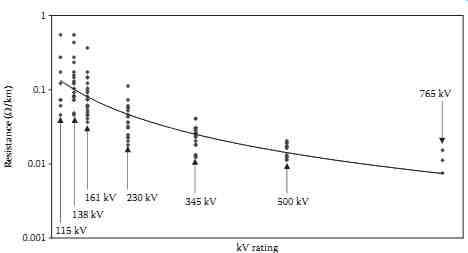
FIG. 12 Range of transmission line resistance in major kV-rating classes
for the U.S. electric power grid infrastructure, with a trend line indicating
common conductor resistances used at each design voltage. The lower resistance
for the higher voltage lines will also cause proportionately larger GIC
flows.
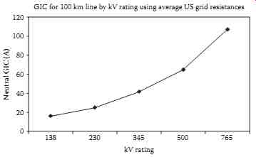
FIG. 13 Average neutral GIC flows versus kV rating for a 100 km demonstration
transmission circuit.
Most power grids are highly complex networks with numerous circuits or paths and transformers for GIC to flow through. This requires the application of highly sophisticated network and electromagnetic coupling models to determine the magnitude and path of GIC throughout the complex power grid.
However, for the purposes of illustrating the impact of power system design, a review will be provided using a single transmission line terminated at each end with a single transformer to ground connection. To illustrate the differences that can occur in levels of GIC flow at higher voltage levels, the simple demonstration circuit have also been developed at 138, 230, 345, 500, and 765 kV, which are common grid voltages used in the United States and Canada. In Europe, voltages of 130, 275, and 400 kV are commonly used for the bulk power grid infrastructures. For these calculations, a uniform 1.0 V/km geo-electric field disturbance conditions are used, which means that the change in GIC levels will result from changes in the power grid resistances alone. Also for uniform comparison purposes, a 100 km long line is used in all kV rating cases.
FIG. 13 illustrates the comparison of GIC flows that would result for various U.S. infrastructure power grid kV ratings using the simple circuit and a uniform 1.0 V/km geo-electric field disturbance.
In complex networks, such as those in the United States, some scatter from this trend line is possible due to normal variations in circuit parameters such as line resistances that can occur in the overall population of infrastructure assets. Further, this was an analysis of simple "one-line" topology network, whereas real power grid networks have highly complex topologies, span large geographic regions, and present numerous paths for GIC flow, all of which tend to increase total GIC flows. Even this limited demonstration tends to illustrate that the power grid infrastructures of large grids in the United States and other locations of the world are increasingly exposed to higher GIC flows due to design changes that have resulted in reduced circuit resistance. Compounding this risk further, the higher kV portions of the network handle the largest bulk power flows and form the backbone of the grid. Therefore the increased GIC risk is being placed at the most vital portions of this critical infrastructure. In the United States, 345, 500, and 765 kV transmission systems are widely spread throughout the United States and especially concentrated in areas of the United States with high population densities.
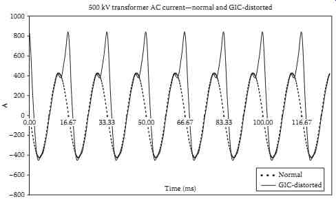
FIG. 14 500 kV simple demonstration circuit simulation results-transformer
AC currents and distortion due to GIC.500 kV transformer AC current-normal
and GIC-distorted.
One of the best ways to illustrate the operational impacts of large GIC flows is to review the way in which the GIC can distort the AC output of a large power transformer due to half-cycle saturation. Under severe geomagnetic storm conditions, the levels of geo-electric field can be many times larger than the uniform 1.0 V/km used in the prior calculations. Under these conditions, even larger GIC flows are possible. For example, in FIG. 14, the normal AC current waveform in the high voltage winding of a 500 kV transformer under normal load conditions is shown (~300 A-rms, ~400 A-peak). With a large GIC flow in the transformer, the transformer experiences extreme saturation of the magnetic core for one-half of the AC cycle (half-cycle saturation). During this half-cycle of saturation, the magnetic core of the transformer draws an extremely large and distorted AC current from the power grid. This com bines with the normal AC load current producing the highly distorted asymmetrically peaky waveform that now flows in the transformer. As shown, AC current peaks that are present are nearly twice as large compared to normal current for the transformer under this mode of operation. This highly distorted waveform is rich in both even and odd harmonics, which are injected into the system and can cause mis-operations of sensors and protective relays throughout the network.
The design of transformers also acts to further compound the impacts of GIC flows in the high-voltage portion of the power grid. While proportionately larger GIC flows occur in these large high-voltage trans formers, the larger high-voltage transformers are driven into saturation at the same few amperes of GIC exposure as those of lower-voltage transformers. More ominously, another compounding of risk occurs as these higher kV-rated transformers produce proportionately higher power system impacts than comparable lower-voltage transformers. As shown in FIG. 15, because reactive power loss in a transformer is a function of the operating voltage, the higher kV-rated transformers will also exhibit proportionately higher reactive power losses due to GIC. For example, a 765 kV transformer will have approximately six times larger reactive power losses for the same magnitude of GIC flow as that of a 115 kV transformer.
All transformers on the network can be exposed to similar conditions simultaneously due to the wide geographic extent of most disturbances. This means that the network needs to supply an extremely large amount of reactive power to each of these transformers or voltage collapse of the network could occur.
The combination of voltage regulation stress, which occurs simultaneously with the loss of key elements due to relay misoperations, can rapidly escalate to widespread progressive collapse of the exposed inter connected network. An example of these threat conditions can be provided for the U.S. power grid for extreme but plausible geomagnetic storm conditions.
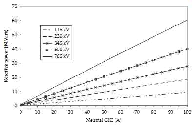
FIG. 15 Comparison of the reactive power losses through transformers
of increasing kV rating versus increasing levels of GIC flow. Higher
kV-rated transformers will produce proportionately larger reactive power
consumption on the grid compared to the same level of GIC flow in lower
kV transformers.
7. Extreme Geomagnetic Disturbance Events: Observational Evidence
Neither the space weather community nor the power industry has fully understood these design implications. The application of detailed simulation models has provided tools for forensic analysis of recent storm activity and when adequately validated can be readily applied to examine impacts due to historically large storms. Some of the first reports of operational impacts to power systems date back to the early 1940s and the level of impacts have progressively become more frequent and significant as growth and development of technology has occurred in this infrastructure. In more contemporary times, major power system impacts in the United States have occurred in storms in 1957, 1958, 1968, 1970, 1972, 1974, 1979, 1982, 1983, and 1989 and several times in 1991. Both empirical and model extrapolations provide some perspective on the possible consequences of storms on present-day infrastructures.
Historic records of geomagnetic disturbance conditions and, more important, geo-electric field measurements provide a perspective on the ultimate driving force that can produce large GIC flows in power grids. Because geo-electric fields and resulting GIC are caused by the rate of change of the geo magnetic field, one of the most meaningful methods to measure the severity of impulsive geomagnetic field disturbances is by the magnitude of the geomagnetic field change per minute, measured in nanoteslas per minute (nT/min). For example, the regional disturbance intensity that triggered the Hydro Quebec collapse during the March 13, 1989 storm only reached an intensity of 479 nT/min. Large numbers of power system impacts in the United States were also observed for intensities that ranged from 300 to 600 nT/min during this storm. However, the most severe rate of change in the geomagnetic field observed during this storm reached a level of ~2000 nT/min over the lower Baltic. The last such disturbance with an intensity of ~2000 nT/min over North America was observed during a storm on August 4, 1972 when the power grid infrastructure was less than 40% of its current size.
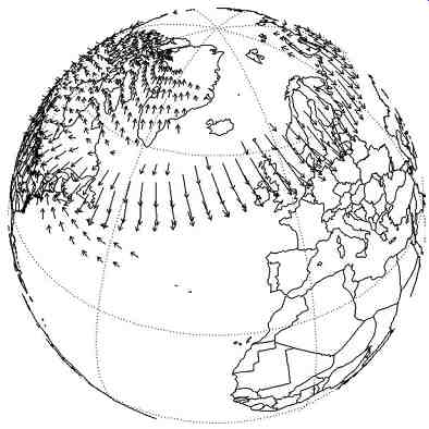
FIG. 16 Extensive westward electrojet-driven geomagnetic field disturbances
at time 22:00UT on March 13, 1989.
Data assimilation models provide further perspectives on the intensity and geographic extent of the intense dB/dt of the March 1989 Superstorm. FIG. 16 provides a synoptic map of the ground-level geomagnetic field disturbance regions observed at time 22:00UT. The previously mentioned lower Baltic region observations are embedded in an enormous westward electrojet complex during this period of time. Simultaneously with this intensification of the westward electrojet, an intensification of the eastward electrojet occupies a region across mid-latitude portions of the western United States. The features of the westward electrojet extend longitudinally ~120° and have a north-south cross-section ranging as much as 5°-10° in latitude.
Older storms provide even further guidance on the possible extremes of these specific electrojet-driven disturbance processes. A remarkable set of observations was conducted on rail communication circuits in Sweden that extend back nearly 80 years. These observations provide key evidence that allow for estimation of the geomagnetic disturbance intensity of historically important storms in an era where geomagnetic observatory data is unavailable. During a similarly intense westward electrojet disturbance on July 13-14, 1982, a ~100 km length communication circuit from Stockholm to Torreboda measured a peak geo-potential of 9.1 V/km (Lindahl). Simultaneous measurements at nearby Lovo observatory in central Sweden measured a dB/dt intensity of ~2600 nT/min at 24:00 UT on July 13. FIG. 17 shows the delta Bx observed at BFE and Lovo during the peak disturbance times on July 13 and for comparison purposes the delta Bx observed at BFE during the large substorm on March 13, 1989. This illustrates that the comparative level of delta Bx is twice as large for the July 13, 1982 event than that observed on March 13, 1989. The large delta Bx of >4000 nT for the July 1982 disturbance suggests that these large field deviations are capable of producing even larger dB/dt impulses should faster onset or collapse of the Bx field occur over the region.
As previously discussed, unprecedented power system impacts were observed in North America on March 13-14, 1989 for storm intensities that reached levels of approximately 300-600 nT/min.
However, the investigation of very large storms indicates that storm intensities over many of these same U.S. regions could be as much as 4-10 times larger. These megastorms appear from historic data to be probable on a 1-in-50 to 1-in-100 year timeframe. Modern critical infrastructures have not as-yet been exposed to storms of this size. This increase in storm intensity causes a nearly proportional increase in resulting stress to power grid operations. These storms also have a footprint that can simultaneously threaten large geographic regions and can therefore plausibly trigger large regions of grid collapse.
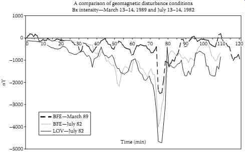
FIG. 17 Comparison of observed delta Bx at Lovo and BFE on July 13-14,
1982, and March 13, 1989, electrojet intensification events.
8. Power Grid Simulations for Extreme Disturbance Events
Based upon these extreme disturbance events, a series of simulations were conducted for the entire U.S. power grid using electrojet-driven disturbance scenarios with the disturbance at 50° geomagnetic latitude and at disturbance strengths of 2400, 3600, and 4800 nT/min. The electrojet disturbance footprint was also positioned over North America with the previously discussed longitudinal dimensions of a large westward electrojet disturbance. This extensive longitudinal structure will simultaneously expose a large portion of the U.S. power grid.
In this analysis of disturbance impacts, the level of cumulative increased reactive demands (MVars) across the U.S. power grid provides one of the more useful measures of overall stress on the network.
This cumulative MVar stress was also determined for the March 13, 1989 storm for the U.S. power grid, which was estimated using the current system model as reaching levels of ~7000-8000 MVars at times 21:44-21:57 UT. At these times, corresponding dB/dt levels in mid-latitude portions of the United States reached 350-545 nT/min as measured at various U.S. observatories. This provides a comparison bench mark that can be used to either compare absolute MVar levels or, the relative MVar level increases for the more severe disturbance scenarios. The higher intensity disturbances of 2400-4800 nT/min will have a proportionate effect on levels of GIC in the exposed network. GIC levels more than five times larger than those observed during the aforementioned periods in the March 1989 storm would be a probable. With the increase in GIC, a linear and proportionate increase in other power system impacts is likely. For example, transformer MVar demands increase with increases in transformer GIC. As larger GICs cause greater degrees of transformer saturation, the harmonic order and magnitude of distortion currents increase in a more complex manner with higher GIC exposures. In addition, greater numbers of transformers would experience sufficient GIC exposure to be driven into saturation, as generally higher and more widely experienced GIC levels would occur throughout the extensive exposed power grid infrastructure.
FIG. 18 provides a comparison summary of the peak cumulative MVar demands that are estimated for the U.S. power grid for the March 89 storm, and for the 2400, 3600, and 4800 nT/min disturbances at the different geomagnetic latitudes. As shown, all of these disturbance scenarios are far larger in magnitude than the levels experienced on the U.S. grid during the March 1989 Superstorm.
All reactive demands for the 2400-4800 nT/min disturbance scenarios would produce unprecedented in size reactive demand increases for the U.S. grid. The comparison with the MVar demand from the March 1989 Superstorm further indicates that even the 2400 nT/min disturbance scenarios would pro duce reactive demand levels at all of the latitudes that would be approximately six times larger than those estimated in March 1989. At the 4800 nT/min disturbance levels, the reactive demand is estimated, in total, to exceed 100,000 MVars. While these large reactive demand increases are calculated for illustration purposes, impacts on voltage regulation and probable large-scale voltage collapse across the network could conceivably occur at much lower levels.
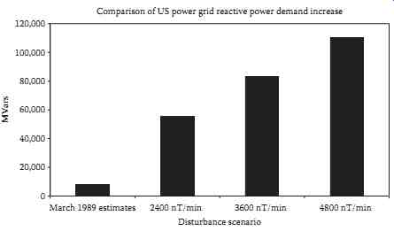
FIG. 18 Comparison of estimated U.S. power grid reactive demands for
the March 13, 1989, Superstorm and 2400, 3600, and 4800 nT/min disturbance
scenarios at 50° geomagnetic latitude position over the United States.
This disturbance environment was further adapted to produce a footprint and onset progression that would be more geo-spatially typical of an electrojet-driven disturbance, using both the March 13, 1989 and July 13, 1982 storms as a template for the electrojet pattern. For this scenario, the intensity of the disturbance is decreased as it progresses from the eastern to western United States. The eastern portions of the United States are exposed to a 4800 nT/min disturbance intensity, while, west of the Mississippi, the disturbance intensity decreases to only 2400 nT/min. The extensive reactive power increase and extensive geographic boundaries of impact would be expected to trigger large-scale progressive collapse conditions, similar to the mode in which the Hydro Quebec collapse occurred. The most probable regions of expected power system collapse can be estimated based upon the GIC levels and reactive demand increases in combination with the disturbance criteria as it applies to the U.S. power pools. FIG. 19 provides a map of the peak GIC flows in the U.S. power grid (size of circle at each node indicates relative GIC intensity) and estimated boundaries of regions that likely could experience system collapse due to this disturbance scenario. This example shows one of many possible scenarios for how a large storm could unfold.
While these complex models have been rigorously tested and validated, this is an exceedingly complex task with uncertainties that can easily be as much as a factor of 2. However, just empirical evidence alone suggests that power grids in North America that were challenged to collapse for storms of 400-600 nT/min over a decade ago are not likely to survive the plausible but rare disturbances of 2000-5000 nT/min that long-term observational evidence indicates have occurred before and therefore may be likely to occur again. Because large power system catastrophes due to space weather are not a zero probability event and because of the large-scale consequences of a major power grid blackout, it is important to discuss the potential societal and economic impacts of such an event should it ever reoccur.
The August 14, 2003 U.S. Blackout event provides a good case study, the utilities and various municipal organizations should be commended for the rapid and orderly restoration efforts that occurred.
However, it should also acknowledge that in many respects this blackout occurred during highly optimal conditions, that were somewhat taken for granted and should not be counted upon in future blackouts. For example, an outage on January 14 rather than August 14 could have meant coincident cold weather conditions. Under these conditions, breakers and equipment at substations and power plants can be more difficult to reenergize when they become cold. Geomagnetic storms as previously discussed can also permanently damage key transformers on the grid which further burdens the restoration process, delays could rapidly cause serious public health and safety concerns.
Because of the possible large geographic lay-down of a severe storm event and resulting power grid collapse, the ability to provide meaningful emergency aid and response to an impacted population that may be in excess of 100 million people will be a difficult challenge. Even basic necessities such as potable water and replenishment of foods may need to come from boundary regions that are unaffected and these unaffected regions could be very remote to portions of the impacted U.S. population centers.
As previously suggested, adverse terrestrial weather conditions could cause further complications in restoration and re-supply logistics.
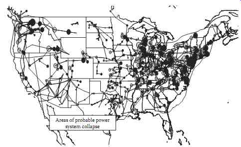
FIG. 19 Regions of large GIC flows and possible power system collapse
due to a 4800 nT/min disturbance scenario.
9. Conclusions
Contemporary models of large power grids and the electromagnetic coupling to these infrastructures by the geomagnetic disturbance environment have matured to a level in which it is possible to achieve very accurate benchmarking of storm geomagnetic observations and the resulting GIC. As abilities advance to model the complex interactions of the space environment with the electric power grid infra structures, the ability to more rigorously quantify the impacts of storms on these critical systems also advances. This quantification of impacts due to extreme space weather events is leading to the recognition that geomagnetic storms are an important threat that has not been well recognized in the past.
Also see...
The Day the Sun Brought Darkness | NASA
solarstorms.org---A Conflagration of Storms