AMAZON multi-meters discounts AMAZON oscilloscope discounts
This guide is an introduction to the young and fast-growing field of data mining (also known as knowledge discovery from data, or KDD for short). The guide focuses on fundamental data mining concepts and techniques for discovering interesting patterns from data in various applications. In particular, we emphasize prominent techniques for developing effective, efficient, and scalable data mining tools.
This section is organized as follows. In Section 1, you will learn why data mining is in high demand and how it is part of the natural evolution of information technology.
Section 2 defines data mining with respect to the knowledge discovery process. Next, you will learn about data mining from many aspects, such as the kinds of data that can be mined (Section 3), the kinds of knowledge to be mined (Section 4), the kinds of technologies to be used (Section 5), and targeted applications (Section 6). In this way, you will gain a multidimensional view of data mining. Finally, Section 7 outlines major data mining research and development issues.
1. Why Data Mining?
Necessity, who is the mother of invention. – Plato
We live in a world where vast amounts of data are collected daily. Analyzing such data is an important need. Section 1.1 looks at how data mining can meet this need by providing tools to discover knowledge from data. In Section 1.2, we observe how data mining can be viewed as a result of the natural evolution of information technology.
1.1 Moving toward the Information Age
"We are living in the information age" is a popular saying; however, we are actually living in the data age. Terabytes or petabytes [A petabyte is a unit of information or computer storage equal to 1 quadrillion bytes, or a thousand terabytes, or 1million gigabytes.] of data pour into our computer networks, the World Wide Web (WWW), and various data storage devices every day from business, society, science and engineering, medicine, and almost every other aspect of daily life.
This explosive growth of available data volume is a result of the computerization of our society and the fast development of powerful data collection and storage tools.
Businesses worldwide generate gigantic data sets, including sales transactions, stock trading records, product descriptions, sales promotions, company profiles and performance, and customer feedback. For example, large stores, such as Wal-Mart, handle hundreds of millions of transactions per week at thousands of branches around the world. Scientific and engineering practices generate high orders of petabytes of data in a continuous manner, from remote sensing, process measuring, scientific experiments, system performance, engineering observations, and environment surveillance.
Global backbone telecommunication networks carry tens of petabytes of data traffic every day. The medical and health industry generates tremendous amounts of data from medical records, patient monitoring, and medical imaging. Billions of Web searches supported by search engines process tens of petabytes of data daily. Communities and social media have become increasingly important data sources, producing digital pictures and videos, blogs, Web communities, and various kinds of social networks. The list of sources that generate huge amounts of data is endless.
This explosively growing, widely available, and gigantic body of data makes our time truly the data age. Powerful and versatile tools are badly needed to automatically uncover valuable information from the tremendous amounts of data and to transform such data into organized knowledge. This necessity has led to the birth of data mining.
The field is young, dynamic, and promising. Data mining has and will continue to make great strides in our journey from the data age toward the coming information age.
Example 1: Data mining turns a large collection of data into knowledge. A search engine (e.g., Google) receives hundreds of millions of queries every day. Each query can be viewed as a transaction where the user describes her or his information need. What novel and useful knowledge can a search engine learn from such a huge collection of queries collected from users over time? Interestingly, some patterns found in user search queries can disclose invaluable knowledge that cannot be obtained by reading individual data items alone. For example, Google's Flu Trends uses specific search terms as indicators of flu activity. It found a close relationship between the number of people who search for flu-related information and the number of people who actually have flu symptoms. A pattern emerges when all of the search queries related to flu are aggregated. Using aggregated Google search data, Flu Trends can estimate flu activity up to two weeks faster than traditional systems can.
This example shows how data mining can turn a large collection of data into knowledge that can help meet a current global challenge.
1.2 Data Mining as the Evolution of Information Technology
Data mining can be viewed as a result of the natural evolution of information technology. The database and data management industry evolved in the development of several critical functionalities (FIG. 1): data collection and database creation, data management (including data storage and retrieval and database transaction processing), and advanced data analysis (involving data warehousing and data mining). The early development of data collection and database creation mechanisms served as a prerequisite for the later development of effective mechanisms for data storage and retrieval, as well as query and transaction processing. Nowadays numerous database systems offer query and transaction processing as common practice. Advanced data analysis has naturally become the next step.
================
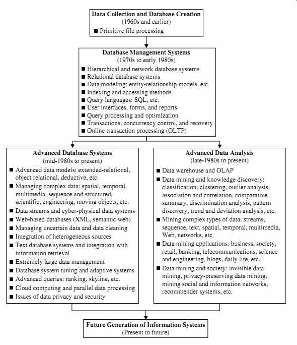
FIG. 1 The evolution of database system technology.
Data Collection and Database Creation (1960s and earlier)
Primitive file processing
Database Management Systems (1970s to early 1980s)
Hierarchical and network database systems
Relational database systems
Data modeling: entity-relationship models, etc.
Indexing and accessing methods
Query languages: SQL, etc.
User interfaces, forms, and reports
Query processing and optimization
Transactions, concurrency control, and recovery
Online transaction processing (OLTP)
Advanced Database Systems (mid-1980s to present)
Advanced data models: extended-relational, object relational, deductive, etc.
Managing complex data: spatial, temporal, multimedia, sequence and structured, scientific, engineering, moving objects, etc.
Data streams and cyber-physical data systems Web-based databases (XML, semantic web) Managing uncertain data and data cleaning Integration of heterogeneous sources Text database systems and integration with information retrieval Extremely large data management Database system tuning and adaptive systems Advanced queries: ranking, skyline, etc.
Cloud computing and parallel data processing Issues of data privacy and security
Advanced Data Analysis (late- 1980s to present)
Data warehouse and OLAP Data mining and knowledge discovery:
classification, clustering, outlier analysis, association and correlation, comparative summary, discrimination analysis, pattern discovery, trend and deviation analysis, etc.
Mining complex types of data: streams, sequence, text, spatial, temporal, multimedia, Web, networks, etc.
Data mining applications: business, society, retail, banking, telecommunications, science and engineering, blogs, daily life, etc.
Data mining and society: invisible data mining, privacy-preserving data mining, mining social and information networks, recommender systems, etc.
Future Generation of Information Systems (Present to future)
================
Since the 1960s, database and information technology has evolved systematically from primitive file processing systems to sophisticated and powerful database systems.
The research and development in database systems since the 1970s progressed from early hierarchical and network database systems to relational database systems (where data are stored in relational table structures; see Section 3.1), data modeling tools, and indexing and accessing methods. In addition, users gained convenient and flexible data access through query languages, user interfaces, query optimization, and transaction management. Efficient methods for online transaction processing (OLTP), where a query is viewed as a read-only transaction, contributed substantially to the evolution and wide acceptance of relational technology as a major tool for efficient storage, retrieval, and management of large amounts of data.
After the establishment of database management systems, database technology moved toward the development of advanced database systems, data warehousing, and data mining for advanced data analysis and web-based databases. Advanced database systems, for example, resulted from an upsurge of research from the mid-1980s onward.
These systems incorporate new and powerful data models such as extended-relational, object-oriented, object-relational, and deductive models. Application-oriented database systems have flourished, including spatial, temporal, multimedia, active, stream and sensor, scientific and engineering databases, knowledge bases, and office information bases. Issues related to the distribution, diversification, and sharing of data have been studied extensively.
Advanced data analysis sprang up from the late 1980s onward. The steady and dazzling progress of computer hardware technology in the past three decades led to large supplies of powerful and affordable computers, data collection equipment, and storage media. This technology provides a great boost to the database and information industry, and it enables a huge number of databases and information repositories to be available for transaction management, information retrieval, and data analysis. Data can now be stored in many different kinds of databases and information repositories.
One emerging data repository architecture is the data warehouse (Section 3.2).
This is a repository of multiple heterogeneous data sources organized under a unified schema at a single site to facilitate management decision making. Data warehouse technology includes data cleaning, data integration, and online analytical processing (OLAP)-that is, analysis techniques with functionalities such as summarization, consolidation, and aggregation, as well as the ability to view information from different angles. Although OLAP tools support multidimensional analysis and decision making, additional data analysis tools are required for in-depth analysis-for example, data mining tools that provide data classification, clustering, outlier/anomaly detection, and the characterization of changes in data over time.
Huge volumes of data have been accumulated beyond databases and data ware houses. During the 1990s, the World Wide Web and web-based databases (e.g., XML databases) began to appear. Internet-based global information bases, such as the WWW and various kinds of interconnected, heterogeneous databases, have emerged and play a vital role in the information industry. The effective and efficient analysis of data from such different forms of data by integration of information retrieval, data mining, and information network analysis technologies is a challenging task.
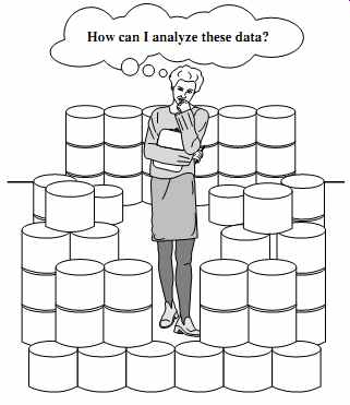
FIG. 2 The world is data rich but information poor.
In summary, the abundance of data, coupled with the need for powerful data analysis tools, has been described as a data rich but information poor situation (FIG. 2). The fast-growing, tremendous amount of data, collected and stored in large and numerous data repositories, has far exceeded our human ability for comprehension without powerful tools. As a result, data collected in large data repositories become "data tombs"-data archives that are seldom visited. Consequently, important decisions are often made based not on the information-rich data stored in data repositories but rather on a decision maker's intuition, simply because the decision maker does not have the tools to extract the valuable knowledge embedded in the vast amounts of data. Efforts have been made to develop expert system and knowledge-based technologies, which typically rely on users or domain experts to manually input knowledge into knowledge bases.
Unfortunately, however, the manual knowledge input procedure is prone to biases and errors and is extremely costly and time consuming. The widening gap between data and information calls for the systematic development of data mining tools that can turn data tombs into "golden nuggets" of knowledge.
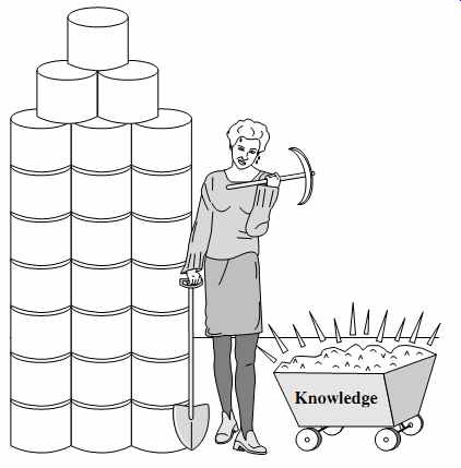
FIG. 3 Data mining-searching for knowledge (interesting patterns) in data.
2. What Is Data Mining?
It is no surprise that data mining, as a truly interdisciplinary subject, can be defined in many different ways. Even the term data mining does not really present all the major components in the picture. To refer to the mining of gold from rocks or sand, we say gold mining instead of rock or sand mining. Analogously, data mining should have been more appropriately named "knowledge mining from data," which is unfortunately somewhat long. However, the shorter term, knowledge mining may not reflect the emphasis on mining from large amounts of data. Nevertheless, mining is a vivid term characterizing the process that finds a small set of precious nuggets from a great deal of raw material (FIG. 3). Thus, such a misnomer carrying both "data" and "mining" became a popular choice. In addition, many other terms have a similar meaning to data mining-for example, knowledge mining from data, knowledge extraction, data/pattern analysis, data archaeology, and data dredging.
Many people treat data mining as a synonym for another popularly used term, knowledge discovery from data, or KDD, while others view data mining as merely an essential step in the process of knowledge discovery. The knowledge discovery process is shown in FIG. 4 as an iterative sequence of the following steps:
1. Data cleaning (to remove noise and inconsistent data)
2. Data integration (where multiple data sources may be combined)3
3. Data selection (where data relevant to the analysis task are retrieved from the database)
4. Data transformation (where data are transformed and consolidated into forms appropriate for mining by performing summary or aggregation operations)4
5. Data mining (an essential process where intelligent methods are applied to extract data patterns)
6. Pattern evaluation (to identify the truly interesting patterns representing knowledge based on interestingness measures-see Section 4.6)
7. Knowledge presentation (where visualization and knowledge representation techniques are used to present mined knowledge to users)
Steps 1 through 4 are different forms of data preprocessing, where data are prepared for mining. The data mining step may interact with the user or a knowledge base. The interesting patterns are presented to the user and may be stored as new knowledge in the knowledge base.
The preceding view shows data mining as one step in the knowledge discovery pro cess, albeit an essential one because it uncovers hidden patterns for evaluation. However, in industry, in media, and in the research milieu, the term data mining is often used to refer to the entire knowledge discovery process (perhaps because the term is shorter than knowledge discovery from data). Therefore, we adopt a broad view of data mining functionality: Data mining is the process of discovering interesting patterns and knowledge from large amounts of data. The data sources can include databases, data warehouses, the Web, other information repositories, or data that are streamed into the system dynamically.
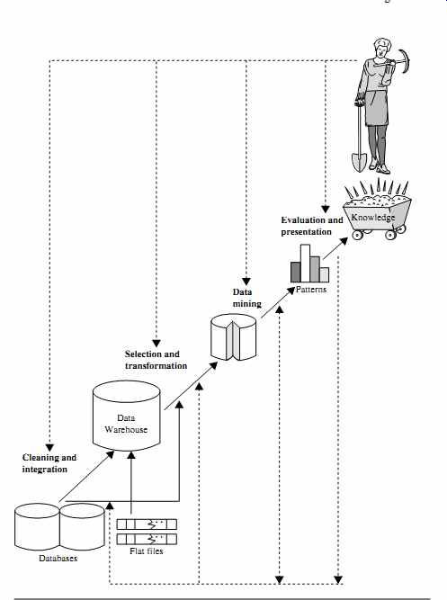
FIG. 4 Data mining as a step in the process of knowledge discovery.
[ A popular trend in the information industry is to perform data cleaning and data integration as a preprocessing step, where the resulting data are stored in a data warehouse. ]
[Sometimes data transformation and consolidation are performed before the data selection process, particularly in the case of data warehousing. Data reduction may also be performed to obtain a smaller representation of the original data without sacrificing its integrity.]
3. What Kinds of Data Can Be Mined?
As a general technology, data mining can be applied to any kind of data as long as the data are meaningful for a target application. The most basic forms of data for mining applications are database data (Section 3.1), data warehouse data (Section 3.2), and transactional data (Section 3.3). The concepts and techniques presented in this guide focus on such data. Data mining can also be applied to other forms of data (e.g., data streams, ordered/sequence data, graph or networked data, spatial data, text data, multimedia data, and the WWW).We present an overview of such data in Section 3.4.
Techniques for mining of these kinds of data are briefly introduced in Section 13. In depth treatment is considered an advanced topic. Data mining will certainly continue to embrace new data types as they emerge.
3.1 Database Data
A database system, also called a database management system (DBMS), consists of a collection of interrelated data, known as a database, and a set of software programs to manage and access the data. The software programs provide mechanisms for defining database structures and data storage; for specifying and managing concurrent, shared, or distributed data access; and for ensuring consistency and security of the information stored despite system crashes or attempts at unauthorized access.
A relational database is a collection of tables, each of which is assigned a unique name. Each table consists of a set of attributes (columns or fields) and usually stores a large set of tuples (records or rows). Each tuple in a relational table represents an object identified by a unique key and described by a set of attribute values. A semantic data model, such as an entity-relationship (ER) data model, is often constructed for relational databases. An ER data model represents the database as a set of entities and their relationships.
Example 2: A relational database for AllElectronics. The fictitious AllElectronics store is used to illustrate concepts throughout this guide. The company is described by the following relation tables: customer, item, employee, and branch. The headers of the tables described here are shown in FIG. 5. (A header is also called the schema of a relation.) The relation customer consists of a set of attributes describing the customer information, including a unique customer identity number (cust ID), customer name, address, age, occupation, annual income, credit information, and category.
Similarly, each of the relations item, employee, and branch consists of a set of attributes describing the properties of these entities.
Tables can also be used to represent the relationships between or among multiple entities. In our example, these include purchases (customer purchases items, creating a sales transaction handled by an employee), items sold (lists items sold in a given transaction), and works at (employee works at a branch of AllElectronics).

FIG. 5 Relational schema for a relational database, AllElectronics.
Relational data can be accessed by database queries written in a relational query language (e.g., SQL) or with the assistance of graphical user interfaces. A given query is transformed into a set of relational operations, such as join, selection, and projection, and is then optimized for efficient processing. A query allows retrieval of specified sub sets of the data. Suppose that your job is to analyze the AllElectronics data. Through the use of relational queries, you can ask things like, "Show me a list of all items that were sold in the last quarter." Relational languages also use aggregate functions such as sum, avg (average), count, max (maximum), and min (minimum). Using aggregates allows you to ask: "Show me the total sales of the last month, grouped by branch," or "How many sales transactions occurred in the month of December?" or "Which salesperson had the highest sales?" When mining relational databases, we can go further by searching for trends or data patterns. For example, data mining systems can analyze customer data to predict the credit risk of new customers based on their income, age, and previous credit information. Data mining systems may also detect deviations-that is, items with sales that are far from those expected in comparison with the previous year. Such deviations can then be further investigated. For example, data mining may discover that there has been a change in packaging of an item or a significant increase in price.
Relational databases are one of the most commonly available and richest information repositories, and thus they are a major data form in the study of data mining.
3.2 Data Warehouses
Suppose that AllElectronics is a successful international company with branches around the world. Each branch has its own set of databases. The president of AllElectronics has asked you to provide an analysis of the company's sales per item type per branch for the third quarter. This is a difficult task, particularly since the relevant data are spread out over several databases physically located at numerous sites.
If AllElectronics had a data warehouse, this task would be easy. A data warehouse is a repository of information collected from multiple sources, stored under a unified schema, and usually residing at a single site. Data warehouses are constructed via a process of data cleaning, data integration, data transformation, data loading, and periodic data refreshing. This process is discussed in Sections 3 and 4. FIG. 6 shows the typical framework for construction and use of a data warehouse for AllElectronics.
To facilitate decision making, the data in a data warehouse are organized around major subjects (e.g., customer, item, supplier, and activity). The data are stored to pro vide information from a historical perspective, such as in the past 6 to 12months, and are typically summarized. For example, rather than storing the details of each sales transaction, the data warehouse may store a summary of the transactions per item type for each store or, summarized to a higher level, for each sales region.
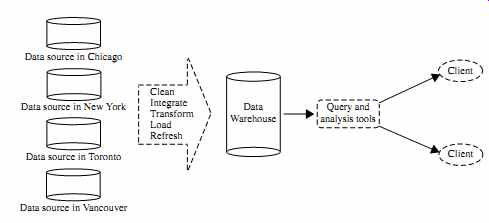
FIG. 6 Typical framework of a data warehouse for AllElectronics.
A data warehouse is usually modeled by a multidimensional data structure, called a data cube, in which each dimension corresponds to an attribute or a set of attributes in the schema, and each cell stores the value of some aggregate measure such as count or sum.sales amount/. A data cube provides a multidimensional view of data and allows the pre-computation and fast access of summarized data.
Example 3: A data cube for AllElectronics. A data cube for summarized sales data of AllElectronics is presented in FIG. 7(a). The cube has three dimensions: address (with city values Chicago, New York, Toronto, Vancouver), time (with quarter values Q1, Q2, Q3, Q4), and item(with item type values home entertainment, computer, phone, security).The aggregate value stored in each cell of the cube is sales amount (in thousands). For example, the total sales for the first quarter, Q1, for the items related to security systems in Vancouver is $400,000, as stored in cell
h. Vancouver,Q1, security
i. Additional cubes may be used to store aggregate sums over each dimension, corresponding to the aggregate values obtained using different SQL group-bys (e.g., the total sales amount per city and quarter, or per city and item, or per quarter and item, or per each individual dimension).
By providing multidimensional data views and the pre-computation of summarized data, data warehouse systems can provide inherent support for OLAP. Online analytical processing operations make use of background knowledge regarding the domain of the data being studied to allow the presentation of data at different levels of abstraction.
Such operations accommodate different user viewpoints. Examples of OLAP operations include drill-down and roll-up, which allow the user to view the data at differing degrees of summarization, as illustrated in FIG. 7(b). For instance, we can drill down on sales data summarized by quarter to see data summarized by month. Similarly, we can roll up on sales data summarized by city to view data summarized by country.
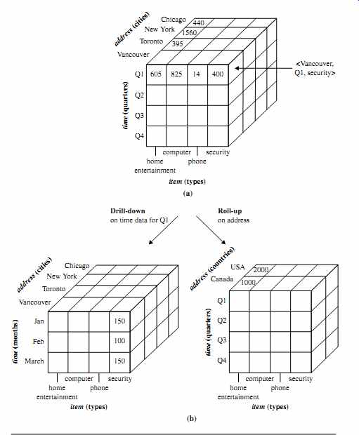
FIG. 7 A multidimensional data cube, commonly used for data warehousing,
(a) showing summarized data for AllElectronics and (b) showing summarized data
resulting from drill-down and roll-up operations on the cube in (a). For improved
readability, only some of the cube cell values are shown.
Although data warehouse tools help support data analysis, additional tools for data mining are often needed for in-depth analysis. Multidimensional data mining (also called exploratory multidimensional data mining) performs data mining in multidimensional space in an OLAP style. That is, it allows the exploration of multiple combinations of dimensions at varying levels of granularity in data mining, and thus has greater potential for discovering interesting patterns representing knowledge. An overview of data warehouse and OLAP technology is provided in Section 4.
Advanced issues regarding data cube computation and multidimensional data mining are discussed in Section 5.
3.3 Transactional Data
In general, each record in a transactional database captures a transaction, such as a customer's purchase, a fight booking, or a user's clicks on a web page. A transaction typically includes a unique transaction identity number (trans ID) and a list of the items making up the transaction, such as the items purchased in the transaction. A transactional database may have additional tables, which contain other information related to the transactions, such as item description, information about the salesperson or the branch, and so on.
Example 4: A transactional database for AllElectronics. Transactions can be stored in a table, with one record per transaction. A fragment of a transactional database for AllElectronics is shown in FIG. 8. From the relational database point of view, the sales table in the figure is a nested relation because the attribute list of item IDs contains a set of items.
Because most relational database systems do not support nested relational structures, the transactional database is usually either stored in a flat file in a format similar to the table in FIG. 8 or unfolded into a standard relation in a format similar to the items sold table in FIG. 5.

FIG. 8 Fragment of a transactional database for sales at AllElectronics.
As an analyst of AllElectronics, you may ask, "Which items sold well together?" This kind of market basket data analysis would enable you to bundle groups of items together as a strategy for boosting sales. For example, given the knowledge that printers are commonly purchased together with computers, you could offer certain printers at a steep discount (or even for free) to customers buying selected computers, in the hopes of selling more computers (which are often more expensive than printers). A traditional database system is not able to perform market basket data analysis. Fortunately, data mining on transactional data can do so by mining frequent item sets, that is, sets of items that are frequently sold together. The mining of such frequent patterns from transactional data is discussed in Sections 6 and 7.
3.4 Other Kinds of Data
Besides relational database data, data warehouse data, and transaction data, there are many other kinds of data that have versatile forms and structures and rather different semantic meanings. Such kinds of data can be seen in many applications: time-related or sequence data (e.g., historical records, stock exchange data, and time-series and bio logical sequence data), data streams (e.g., video surveillance and sensor data, which are continuously transmitted), spatial data (e.g., maps), engineering design data (e.g., the design of buildings, system components, or integrated circuits), hypertext and multi media data (including text, image, video, and audio data), graph and networked data (e.g., social and information networks), and the Web (a huge, widely distributed information repository made available by the Internet). These applications bring about new challenges, like how to handle data carrying special structures (e.g., sequences, trees, graphs, and networks) and specific semantics (such as ordering, image, audio and video contents, and connectivity), and how to mine patterns that carry rich structures and semantics.
Various kinds of knowledge can be mined from these kinds of data. Here, we list just a few. Regarding temporal data, for instance, we can mine banking data for changing trends, which may aid in the scheduling of bank tellers according to the volume of customer traffic. Stock exchange data can be mined to uncover trends that could help you plan investment strategies (e.g., the best time to purchase AllElectronics stock). We could mine computer network data streams to detect intrusions based on the anomaly of message flows, which may be discovered by clustering, dynamic construction of stream models or by comparing the current frequent patterns with those at a previous time.
With spatial data, we may look for patterns that describe changes in metropolitan poverty rates based on city distances from major highways. The relationships among a set of spatial objects can be examined in order to discover which subsets of objects are spatially auto correlated or associated. By mining text data, such as literature on data mining from the past ten years, we can identify the evolution of hot topics in the field. By mining user comments on products (which are often submitted as short text messages), we can assess customer sentiments and understand how well a product is embraced by a market. From multimedia data, we can mine images to identify objects and classify them by assigning semantic labels or tags. By mining video data of a hockey game, we can detect video sequences corresponding to goals. Web mining can help us learn about the distribution of information on the WWW in general, characterize and classify web pages, and uncover web dynamics and the association and other relationships among different web pages, users, communities, and web-based activities.
It is important to keep in mind that, in many applications, multiple types of data are present. For example, in web mining, there often exist text data and multimedia data (e.g., pictures and videos) on web pages, graph data like web graphs, and map data on some web sites. In bioinformatics, genomic sequences, biological networks, and 3-D spatial structures of genomes may coexist for certain biological objects. Mining multiple data sources of complex data often leads to fruitful findings due to the mutual enhancement and consolidation of such multiple sources. On the other hand, it is also challenging because of the difficulties in data cleaning and data integration, as well as the complex interactions among the multiple sources of such data.
While such data require sophisticated facilities for efficient storage, retrieval, and updating, they also provide fertile ground and raise challenging research and implementation issues for data mining. Data mining on such data is an advanced topic. The methods involved are extensions of the basic techniques presented in this guide.
4. What Kinds of Patterns Can Be Mined?
We have observed various types of data and information repositories on which data mining can be performed. Let us now examine the kinds of patterns that can be mined.
There are a number of data mining functionalities. These include characterization and discrimination (Section 4.1); the mining of frequent patterns, associations, and correlations (Section 4.2); classification and regression (Section 4.3); clustering analysis (Section 4.4); and outlier analysis (Section 4.5). Data mining functionalities are used to specify the kinds of patterns to be found in data mining tasks. In general, such tasks can be classified into two categories: descriptive and predictive. Descriptive mining tasks characterize properties of the data in a target data set. Predictive mining tasks perform induction on the current data in order to make predictions.
Data mining functionalities, and the kinds of patterns they can discover, are described below. In addition, Section 4.6 looks at what makes a pattern interesting. Interesting patterns represent knowledge.
4.1 Class/Concept Description: Characterization and Discrimination
Data entries can be associated with classes or concepts. For example, in the AllElectronics store, classes of items for sale include computers and printers, and concepts of customers include bigSpenders and budgetSpenders. It can be useful to describe individual classes and concepts in summarized, concise, and yet precise terms. Such descriptions of a class or a concept are called class/concept descriptions. These descriptions can be derived using (1) data characterization, by summarizing the data of the class under study (often called the target class) in general terms, or (2) data discrimination, by comparison of the target class with one or a set of comparative classes (often called the contrasting classes), or (3) both data characterization and discrimination.
Data characterization is a summarization of the general characteristics or features of a target class of data. The data corresponding to the user-specified class are typically collected by a query. For example, to study the characteristics of software products with sales that increased by 10% in the previous year, the data related to such products can be collected by executing an SQL query on the sales database.
There are several methods for effective data summarization and characterization.
Simple data summaries based on statistical measures and plots are described in Section 2. The data cube-based OLAP roll-up operation (Section 3.2) can be used to perform user-controlled data summarization along a specified dimension. This pro cess is further detailed in Sections 4 and 5, which discuss data warehousing. An attribute-oriented induction technique can be used to perform data generalization and characterization without step-by-step user interaction. This technique is also described in Section 4.
The output of data characterization can be presented in various forms. Examples include pie charts, bar charts, curves, multidimensional data cubes, and multidimensional tables, including crosstabs. The resulting descriptions can also be presented as generalized relations or in rule form (called characteristic rules).
Example 5 Data characterization. A customer relationship manager at AllElectronics may order the following data mining task: Summarize the characteristics of customers who spend more than $5000 a year at AllElectronics. The result is a general profile of these customers, such as that they are 40 to 50 years old, employed, and have excellent credit ratings. The data mining system should allow the customer relationship manager to drill down on any dimension, such as on occupation to view these customers according to their type of employment.
Data discrimination is a comparison of the general features of the target class data objects against the general features of objects from one or multiple contrasting classes.
The target and contrasting classes can be specified by a user, and the corresponding data objects can be retrieved through database queries. For example, a user may want to compare the general features of software products with sales that increased by 10% last year against those with sales that decreased by at least 30% during the same period. The methods used for data discrimination are similar to those used for data characterization.
"How are discrimination descriptions output?" The forms of output presentation are similar to those for characteristic descriptions, although discrimination descriptions should include comparative measures that help to distinguish between the target and contrasting classes. Discrimination descriptions expressed in the form of rules are referred to as discriminant rules.
Example 6: Data discrimination. A customer relationship manager at AllElectronics may want to compare two groups of customers-those who shop for computer products regularly (e.g., more than twice a month) and those who rarely shop for such products (e.g., less than three times a year). The resulting description provides a general comparative profile of these customers, such as that 80% of the customers who frequently purchase computer products are between 20 and 40 years old and have a university education, whereas 60% of the customers who infrequently buy such products are either seniors or youths, and have no university degree. Drilling down on a dimension like occupation, or adding a new dimension like income level, may help to find even more discriminative features between the two classes.
Concept description, including characterization and discrimination, is described in Section 4.
4.2 Mining Frequent Patterns, Associations, and Correlations
Frequent patterns, as the name suggests, are patterns that occur frequently in data.
There are many kinds of frequent patterns, including frequent item sets, frequent sub sequences (also known as sequential patterns), and frequent substructures. A frequent item set typically refers to a set of items that often appear together in a transactional data set-for example, milk and bread, which are frequently bought together in grocery stores by many customers. A frequently occurring subsequence, such as the pattern that customers, tend to purchase first a laptop, followed by a digital camera, and then a memory card, is a (frequent) sequential pattern. A substructure can refer to different structural forms (e.g., graphs, trees, or lattices) that may be combined with item sets or subsequences. If a substructure occurs frequently, it is called a (frequent) structured pattern. Mining frequent patterns leads to the discovery of interesting associations and correlations within data.
Example 7: Association analysis. Suppose that, as a marketing manager at AllElectronics, you want to know which items are frequently purchased together (i.e., within the same transaction). An example of such a rule, mined from the AllElectronics transactional database, is buys.X, "computer"/)buys.X, "software"/ [support D 1%, confidence D 50%], where X is a variable representing a customer. A confidence, or certainty, of 50% means that if a customer buys a computer, there is a 50% chance that she will buy software as well. A 1% support means that 1% of all the transactions under analysis show that computer and software are purchased together. This association rule involves a single attribute or predicate (i.e., buys) that repeats. Association rules that contain a single predicate are referred to as single-dimensional association rules. Dropping the predicate notation, the rule can be written simply as "computer )software [1%, 50%]." Suppose, instead, that we are given the AllElectronics relational database related to purchases. A data mining system may find association rules like
age.X, "20..29"/^income.X, "40K..49K"/)buys.X, "laptop"/
[support D 2%, confidence D 60%].
The rule indicates that of the AllElectronics customers under study, 2%are 20 to 29 years old with an income of $40,000 to $49,000 and have purchased a laptop (computer) at AllElectronics. There is a 60% probability that a customer in this age and income group will purchase a laptop. Note that this is an association involving more than one attribute or predicate (i.e., age, income, and buys). Adopting the terminology used in multidimensional databases, where each attribute is referred to as a dimension, the above rule can be referred to as a multidimensional association rule.
Typically, association rules are discarded as uninteresting if they do not satisfy both a minimum support threshold and a minimum confidence threshold. Additional analysis can be performed to uncover interesting statistical correlations between associated attribute-value pairs.
Frequent itemset mining is a fundamental form of frequent pattern mining. The mining of frequent patterns, associations, and correlations is discussed in Sections 6 and 7, where particular emphasis is placed on efficient algorithms for frequent item set mining. Sequential pattern mining and structured pattern mining are considered advanced topics.
4.3 Classification and Regression for Predictive Analysis
Classification is the process of finding a model (or function) that describes and distinguishes data classes or concepts. The model are derived based on the analysis of a set of training data (i.e., data objects for which the class labels are known). The model is used to predict the class label of objects for which the class label is unknown.
"How is the derived model presented?" The derived model may be represented in various forms, such as classification rules (i.e., IF-THEN rules), decision trees, mathematical formulae, or neural networks (FIG. 9).A decision tree is a flowchart-like tree structure, where each node denotes a test on an attribute value, each branch represents an outcome of the test, and tree leaves represent classes or class distributions. Decision trees can easily be converted to classification rules. A neural network, when used for classification, is typically a collection of neuron-like processing units with weighted connections between the units. There are many other methods for constructing classification models, such as naive Bayesian classification, support vector machines, and k-nearest-neighbor classification.
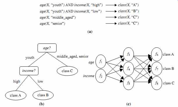
FIG. 9 A classification model can be represented in various forms: (a)
IF-THEN rules, (b) a decision tree, or (c) a neural network.
Whereas classification predicts categorical (discrete, unordered) labels, regression models continuous-valued functions. That is, regression is used to predict missing or unavailable numerical data values rather than (discrete) class labels. The term prediction refers to both numeric prediction and class label prediction. Regression analysis is a statistical methodology that is most often used for numeric prediction, although other methods exist as well. Regression also encompasses the identification of distribution trends based on the available data.
Classification and regression may need to be preceded by relevance analysis, which attempts to identify attributes that are significantly relevant to the classification and regression process. Such attributes will be selected for the classification and regression process. Other attributes, which are irrelevant, can then be excluded from consideration.
Example 8: Classification and regression. Suppose as a sales manager of AllElectronics you want to classify a large set of items in the store, based on three kinds of responses to a sales campaign: good response, mild response and no response. You want to derive a model for each of these three classes based on the descriptive features of the items, such as price, brand, place made, type, and category. The resulting classification should maximally distinguish each class from the others, presenting an organized picture of the data set.
Suppose that the resulting classification is expressed as a decision tree. The decision tree, for instance, may identify price as being the single factor that best distinguishes the three classes. The tree may reveal that, in addition to price, other features that help to further distinguish objects of each class from one another include brand and place made.
Such a decision tree may help you understand the impact of the given sales campaign and design a more effective campaign in the future.
Suppose instead, that rather than predicting categorical response labels for each store item, you would like to predict the amount of revenue that each item will generate during an upcoming sale at AllElectronics, based on the previous sales data. This is an example of regression analysis because the regression model constructed will predict a continuous function (or ordered value.) Sections 8 and 9 discuss classification in further detail. Regression analysis is beyond the scope of this guide. Sources for further information are given in the bibliographic notes.
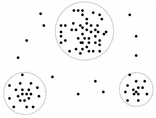
FIG. 10: A 2-D plot of customer data with respect to customer locations
in a city, showing three data clusters.
4.4 Cluster Analysis
Unlike classification and regression, which analyze class-labeled (training) data sets, clustering analyzes data objects without consulting class labels. In many cases, class labeled data may simply not exist at the beginning. Clustering can be used to generate class labels for a group of data. The objects are clustered or grouped based on the principle of maximizing the intra-class similarity and minimizing the interclass similarity. That is, clusters of objects are formed so that objects within a cluster have high similarity in com parison to one another, but are rather dissimilar to objects in other clusters. Each cluster so formed can be viewed as a class of objects, from which rules can be derived. Clustering can also facilitate taxonomy formation, that is, the organization of observations into a hierarchy of classes that group similar events together.
Example 9: Cluster analysis. Cluster analysis can be performed on AllElectronics customer data to identify homogeneous subpopulations of customers. These clusters may represent individual target groups for marketing. FIG. 10 shows a 2-D plot of customers with respect to customer locations in a city. Three clusters of data points are evident.
Cluster analysis forms the topic of Sections 10 and 11.
NEXT>>