AMAZON multi-meters discounts AMAZON oscilloscope discounts
7. Single-Phase Shunt Active Power Filter Topology
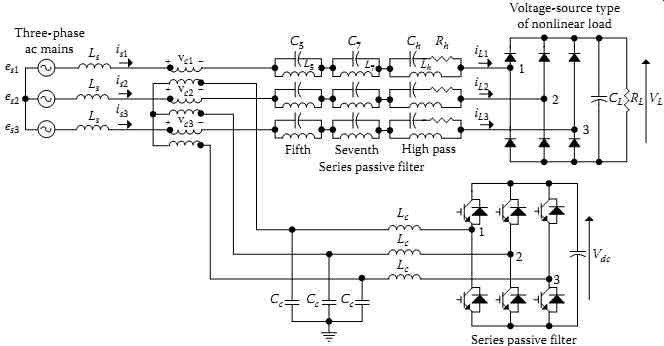
FIG. 44 Three-phase three-wire voltage-fed series hybrid filter.
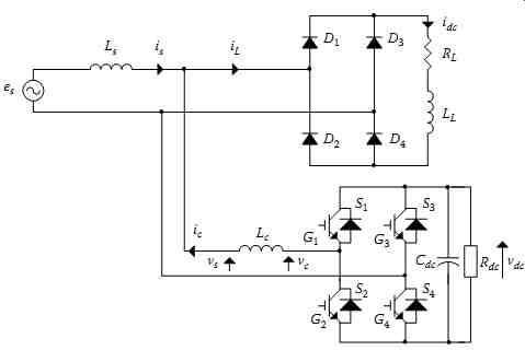
FIG. 45 Configuration of the studied system.
FIG. 45 shows the complete system where the SPSAPF is connected in parallel with a nonlinear load consisting of a single-phase diode rectifier. The SPSAPF consists of a single-phase PWM full-bridge voltage-source inverter, a dc bus capacitor Cdc, and an inductor Lc, which is required to attenuate the high-frequency ripples generated by the voltage-source inverter (VSI). A single-phase diode bridge rectifier feeding a series RL circuit represents the nonlinear load. The converter losses are represented by shunt resistance Rdc connected in parallel to a dc bus capacitor Cdc.
7.1 Extraction of Reference Signals
The performance of an active filter is greatly influenced by the method used for extracting the current reference. There are two control techniques for line current wave shaping in an active filter: the direct current control and the indirect current control. In the direct current control technique, the closed-loop current error is the difference between the desired current ic* and the real current ic at the ac input of the shunt active filter. Whereas, in the indirect current control strategy, the current error is the gap between the source current reference is* and the sensed source current is.
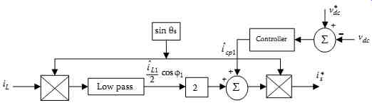
FIG. 46 Indirect current control algorithm of SPSAPF system.
7.1.1 T he Indirect Current Control Technique of SPSHPF
The generation of the reference current is based on the determination of the amplitude of the fundamental active current iLf, which is done with the help of the classic demodulation technique. The nonlinear load current iL is decomposed of the fundamental component iLf and the harmonic components iLh as follows:
where:
ϕ1 is the phase angle of the fundamental load current
θs = wt, w being the mains frequency
ˆiL1 is the peak value of the fundamental current
ˆiLh is the peak value of the hth harmonic load current
ϕh is the angle of the hth harmonic load current
On the other hand, the fundamental current can be divided into two components, namely, fundamental active iLfa = ˆiL1 cos ϕ1 sin θs and fundamental reactive iLfr = ˆiL1 sin ϕ1 cos θs.
This technique allows the compensation of harmonics and reactive power at the same time. The objective is to cancel the harmonics and to compensate for the reactive power; therefore, the reference current for the active filter is* is equal to the load fundamental active current iLfa:
In order to simplify the filtering of the load current iLh, the fundamental component iLfa is transformed into the dc component. Multiplying both sides of Equation 38.19 by sin θs,
This equation shows the presence of a dc component and the ac components of which minimal frequency is equal to twice the frequency network (120 Hz). A low-pass filter, with a relatively low cut-off frequency is used to prevent the high-frequency component. However, it is indispensable to respect a good compromise between the effective filtering of frequencies parasites and the fast dynamics of the extraction algorithm.
The compensator active current ˆicp1 is obtained from the bus voltage regulation loop. The error between the reference value Vdc * and the sensed feedback value Vdc is processed toward a PI controller giving ˆicp1 signal. This current is added to 2*iL filtered, leading the peak value of the reference current. In order to reconstitute the fundamental active reference current, the peak value is multiplied by sin θs. The block diagram that generates is* is shown in FIG. 46.
7.1.2 T he Direct Current Control Technique of SPSHPF
The proposed block diagram of the control algorithm of an active filter with direct current control is shown in FIG. 47.
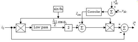
FIG. 47 Direct current control algorithm of SPSAPF system.
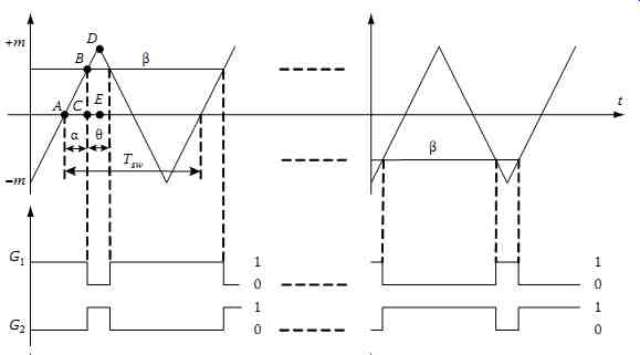
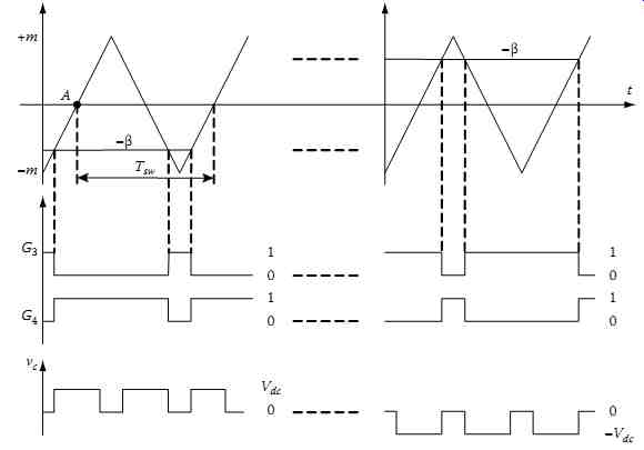
FIG. 48 PWM gating signals generation using U-PWM control technique.
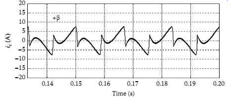
FIG. 49 Modulating signal β.
7.2 Principle of the Unipolar PWM Control
The generation of the U-PWM control pattern is illustrated in FIG. 48. It is based on two comparisons:
(1) between a control signal β and a triangular high-frequency carrier, and (2) between the opposite of the control signal (−β) and the same carrier. A typical waveform of the control signal β is given in FIG. 49. Such a signal, which is slow time-varying in each half-period-wide interval, is generally delivered by a closed-loop PI controller that adjusts continuously the current ic at the input of the active filter to track a current reference ic* such that ...
...where ωs denotes the angular frequency of the mains. The waveform given in FIG. 49 allows compensating both the undesirable harmonics in the source current and the reactive power required by the nonlinear load.
Considering the frequency range of the control signal β and the triangular carrier, one may consider that the modulating signal is practically constant during a switching period Tsw. In this case, referring to FIG. 48, we have ...
…where… d1 and d2 are, respectively, the duty cycles of switches T1 and T3 over one sampling period Tsw ... m is the peak value of the triangular carrier.
One can, thus, deduce the average value of the voltage vc at the input of the inverter over a switching period Tsw:
It should be noted that the average voltage vc Tsw ... is proportional to the control variable β. For operation below the switching frequency, one can assume that the PWM inverter transfer function is equivalent to the constant G.
7.2.1 Harmonic Analysis of Active Power Filter Inverter Input Voltage vc
According to FIG. 48, the voltage vc is an alternating modulated square wave signal. Its frequency is twice the control signal of S1 and S3, and its magnitude is lower than the peak of its fundamental. In the following, let us define vc = vc1 when the standard PWM is used and vc = vc2 when the U-PWM is used.
7.2.2 Harmonic Analysis with Standard PWM (vc = vc1)
Under the assumption that the voltage vc1 remains periodic over a few successive switching cycles, i.e., d1Tsw = constant, by applying the Fourier transform to vc waveform shown in FIG. 50, a first local decomposition is applied to the voltage vc1:
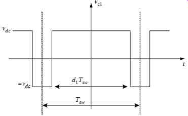
FIG. 50 Voltage waveform of vc1 obtained by B-PWM.
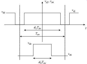
FIG. 51 Voltage waveform of vs2 and vs4 obtained with U-PWM.
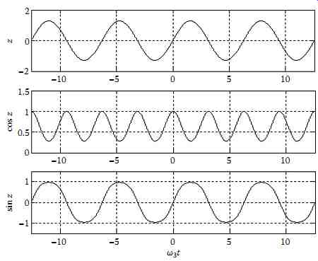
FIG. 52 Waveform of functions z, cos z, and sin z.
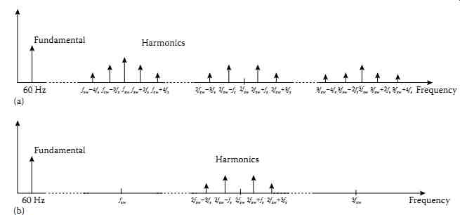
FIG. 53 Comparison between the spectra of the voltage vc obtained by
(a) the B-PWM and (b) the U-PWM.
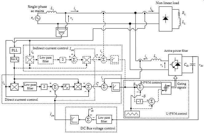
FIG. 54 System block diagram with direct or indirect control blocks
and B-PWM or U-PWM techniques in dashed line.
7.3 PWM's Principle of Gating Signal Generation
The reference supply (harmonic) current obtained from the control algorithm is compared with sensed supply (filter) current. As above, the error signal is fed to a controller having a limiter at its output.
Consequently, the controlling signal β and its opposite −β are compared with a triangular carrier wave resulting in the switching signals to the gates of solid-state switching devices of VSI as shown is FIG. 54.
7.4 Control of Active Power Filter
FIG. 54 shows the complete diagram used for the identification of the active fundamental load current. This diagram includes the direct and indirect current control algorithm implemented with the B-PWM and U-PWM controllers. Besides the estimation of active fundamental load current, a real current reference component is derived from a PI regulator that controls the dc bus voltage of the inverter as shown in FIG. 54. The component is summed to create the demanded reference supply current for the inner current regulator loop.
7.5 Small-Signal Modeling of the Single-Phase Active Power Filter
7.5.1 Averaged Model
By applying the average modeling technique to the filter in FIG. 45, the following state equations are obtained:
7.5.2 Linear Control System
The control system is illustrated in FIG. 54. A successive two-loops strategy is employed. The inner loop embeds an indirect current control technique. Here, and contrarily to the direct control method where the controlled current is the one at the filter input, it is the source current that is sensed and injected in an inner feedback system in order to shape it. This approach allows simplifying considerably the generation of the current reference and offers better dynamics due to the absence of discontinuities in the current reference waveform. The outer loop, which is designed to be enough slower than the inner one for stability considerations, ensures voltage regulations at the dc side of the filter by compensating the power losses in the semiconductors and the reactive elements of the filter (recall that these losses are represented by the fictive resistance Rdc in FIG. 45).
In order to choose adequately the inner and outer regulators, the knowledge of the filter's small-signal transfer functions is required. As noticed in FIG. 54, the determination of the transfer functions, on the basis of which the regulators are calculated, follows two steps.
7.5.2.1 Inner Subsystem Transfer Function
First, the inner control loop is considered. Here, a transfer function relating the inner output variable is to the control input d1 has to be established. This is easily done by applying first small-signal linearization to Equation 38.45. We get ...
....where δx denotes the small-variation of a time variable x around its static value X. Furthermore, the static regime is obtained by setting all the time derivatives and the small variations to zero. It yields ...
Note that the input voltage ̅vs and the load current ̅iL are regarded as disturbance signals in the control design process. Thus, it appears clearly that the inner subsystem exhibits an integrator-like behavior, which makes quite easy the determination of the inner regulator transfer function that would ensure optimal dynamic characteristics to the inner current loop. A typical regulator is a first-order low-pass filter, as it will be demonstrated subsequently. The regulator's parameters are chosen in order to ensure, first, a maximized open-loop gain in the bandwidth and, thus, a minimized current error at the input of the regulator and, second, the attenuation of the current harmonics at multiple switching frequency.
7.5.2.2 Outer Subsystem Transfer Function
The development of the system transfer function for the design of the outer control loop is carried out by taking into account the presence of the inner one. Furthermore, it will be assumed that the inner regulator is suitably chosen, so that the inner controlled variable is follows perfectly the current reference is*: The parameters of the regulator (Ki and τi) are calculated so that the system ensures a fast dynamic response, and the current is of the supply takes a sinusoidal form, and in phase with the voltage. The values of Ki and τi are given in TBL. 1.
7.6 Simulation Results
In order to validate the accuracy of these controllers, the system is simulated using the parameters as given in TBL. 1. The circuit of FIG. 54 was implemented in the Simulink• toolbox of MATLAB under various conditions.
TBL. 1 System Parameters Used for Simulation
7.6.1 Compensation for Direct and Indirect Current Control Techniques Implemented with the Bipolar PWM Controller
The simulation results of the SPSAPF with direct and indirect current control algorithms implemented with the B-PWM controller are presented in FIG. 55a and b, respectively, where load current (iL), the SPSAPF current (ic), the supply voltage (vs), the supply current (is), and the dc bus voltage of the SPSAPF (vdc) are depicted. The harmonic spectra of the supply current before and after compensation with direct and indirect current control schemes implemented with the B-PWM controller are shown in FIG. 56a through c, respectively. The THD of the supply current is reduced from 28.5% before compensation to 10.4% after compensation with the direct current control technique and to 6.3% with the indirect current control technique. These results show that when using indirect current control technique, the current ripple of the supply current has eliminated. Moreover, it is observed that the B-PWM controller suffers from the problem of high-frequency harmonics in the supply current.
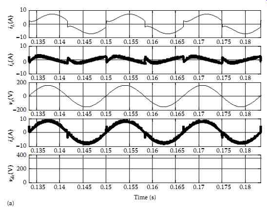
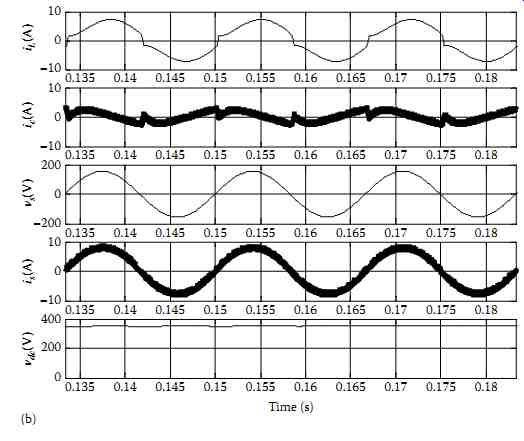
FIG. 55 Steady-state waveforms of the SPSAPF system: (a) direct current
control implemented with the B-PWM, (b) indirect current control implemented
with the B-PWM.
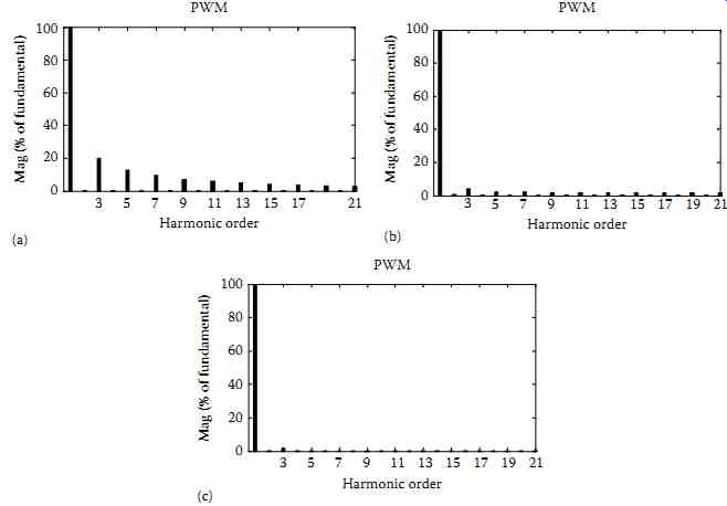 FIG. 56 Spectrum of the source current: (a) before compensation and
after compensation with, (b) direct current control implemented with
the B-PWM, and (c) indirect current control implemented with the B-PWM.
FIG. 56 Spectrum of the source current: (a) before compensation and
after compensation with, (b) direct current control implemented with
the B-PWM, and (c) indirect current control implemented with the B-PWM.
7.6.2 Compensation for These Direct and Indirect Current Techniques Implemented with the Unipolar PWM Controller
FIG. 57a and b show the steady-state operation of the SPSAPF with the direct and indirect current control techniques implemented with the U-PWM controller. The harmonic spectra of the supply current after compensation with direct and indirect current control techniques implemented with the U-PWM controller are shown in FIG. 58a and b, respectively. The THD of the supply current is reduced from 28.5% before compensation to 4.4% after compensation with the direct current control technique and to 1% with the indirect current control technique. In order to show the efficiency of the U-PWM controller regarding the high-frequency content of the supply current, one can compare, as shown in FIG. 59, the harmonic spectra of both techniques. Note that this comparison is made within the vicinities of switching frequencies fsw and 2fsw.
In practice, the loads power demand are usually subject to variations. Hence, it is necessary to examine the performance of the indirect current control technique implemented with the U-PWM controller under such disturbances. FIG. 60 shows the response of the SPSAPF system for a step increase of 100% of the load current at t = 166.7 ms. During the change of load condition, the system maintains unity PF operation and the dc bus voltage of SPSAPF is also regulated to the reference value. These results confirm that by using indirect current control technique with the U-PWM control strategy, substantial improvements have been observed in harmonic content of the supply current as well as on dynamic response of the SPSAPF.
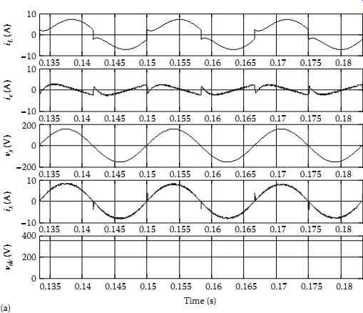
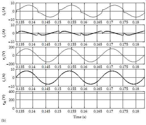
FIG. 57 Steady-state waveforms of the SPSAPF system: (a) direct current
control implemented with the U-PWM, (b) indirect current control implemented
with the U-PWM.
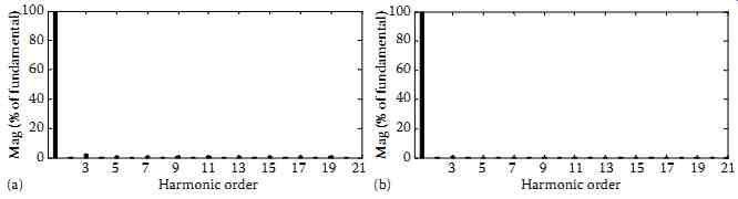
FIG. 58 Spectrum of source current after compensation with (a) direct
current control implemented with the U-PWM and (b) indirect current control
implemented with the U-PWM.
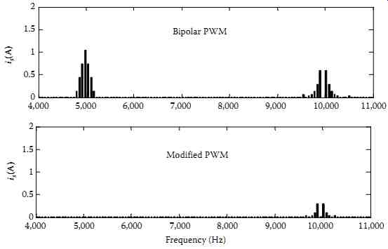
FIG. 59 Spectrum analysis of source currents obtained using indirect
current control with B-PWM and U-PWM.
It is observed that the indirect current control algorithm of SPSAPF implemented with the U-PWM controller is free from switching ripples and high-frequency harmonics in the supply current. The reference supply current is a slowly varying signal (60 Hz), therefore at any instant on the ac cycle, the indirect current controller has exact information about the shape of the supply current and, hence, it takes a desired corrective action to fully compensate the switching ripples in the supply current. The supply current is observed very close to sinusoidal wave and it remains in phase with the supply voltage, therefore unity PF is maintained at ac mains. The SPSAPF supplies the reactive power demand of the load locally and it also compensates its harmonics. The THD of supply current for different control techniques is summarized in TBL. 2.
7.7 Experimental Validation
To experimentally validate the developed model of SPSAPF, various tests are conducted. Both direct and indirect current control techniques with both PWM controllers have been implemented. The experimental setup parameters as a 574 VA diode rectifier is taken as the nonlinear load; the supply voltage is a 110 V, 60 Hz. The SPSAPF is made of 4-IGBT modules IXGH 40 N60 of Ixys. The dc voltage is set at 350 V.
The filter inductor is selected to be 5 mH and the dc bus capacitor is 2000 μF. The switching frequency of the IGBT devices is taken as 5 kHz.
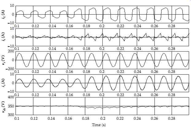
FIG. 60 System response to a 100% step of load increase.
TBL. 2 THD Value of the Compensated Source Current
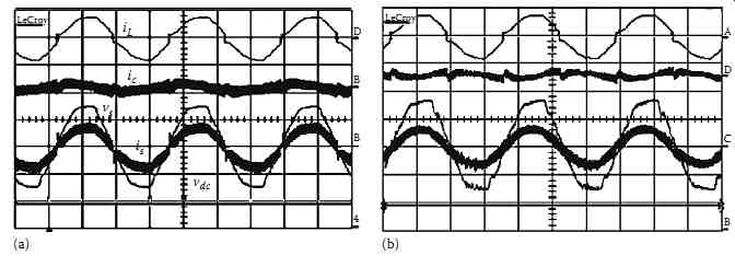
FIG. 61 Steady-state waveforms: (a) direct current control implemented
with the B-PWM and (b) indirect current control implemented with the
B-PWM, vs, [100 V/div], vdc [400 V/div], is [10 A/div], iL [10 A/div]
and ic [10 A/div], time (5 mS/div).
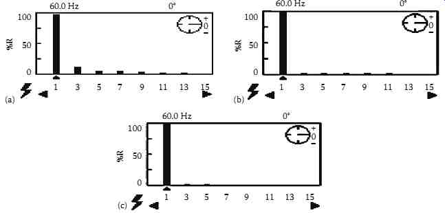
FIG. 62 Spectrum of the source current: (a) before compensation and
after compensation with (b) current control implemented with the B-PWM,
and (c) indirect current control implemented with the B-PWM.
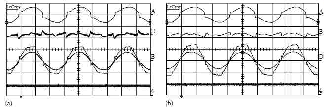
FIG. 63 Steady-state waveforms: (a) direct current control implemented
with the U-PWM and (b) indirect current control implemented with the
U-PWM, vs, [100 V/div], vdc [400 V/div], is [10 A/div], iL [10 A/div]
and ic [10 A/div], Time (5 mS/div).
7.7.1 Compensation for These Direct and Indirect Current Control Techniques Implemented with the Bipolar PWM Controller
The steady-state results of the direct current control technique implemented with the B-PWM controller are shown in FIG. 61a, and the waveforms of the indirect current control technique implemented with the B-PWM controller are shown in FIG. 61b. These results demonstrate the capability of the indirect current control technique to eliminate the ripples. The low-frequency analysis of the load and supply currents is shown in FIG. 62a through c. The THD of this supply current is decreased from 28.83% to 10.9% with the direct current control technique implemented with the B-PWM controller and from 28.83% to 6.7% with the indirect current control technique implemented with the B-PWM controller.
7.7.2 Compensation for These Direct and Indirect Current Control Techniques Implemented with the Unipolar PWM Controller
FIG. 63a and b show the steady-state results of the direct current control technique implemented with the U-PWM controller and the waveforms of the indirect current control technique implemented with the U-PWM controller. These results demonstrate the capability of the U-PWM controller to better compensate the low-frequency harmonics. The low-frequency analysis of supply current is shown in FIG. 64a and b. The THD of this supply current is decreased from 28.83% to 4.9% with the direct current control technique implemented with the U-PWM controller and from 28.83% to 2.2% with the indirect current control technique implemented with the U-PWM controller.
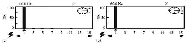
FIG. 64 Spectrum of the source current after compensation with (a)
direct current control implemented with the U-PWM and (b) indirect current
control implemented with the U-PWM.
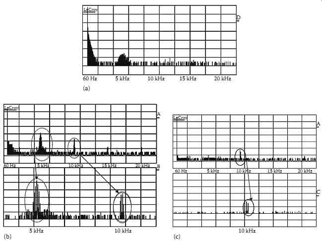
FIG. 65 Source current spectrum covering both low- and high-frequency
components: (a) before compensation and after compensation with, (b)
indirect current control implemented with the B-PWM (top caption amplitude
9.2 dB/div, bottom caption zoom view 5.5 dB/div) and (c) indirect current
control implemented with the U-PWM (top caption amplitude 9.2 dB/div,
bottom caption zoom view 9.2 dB/div).
In order to evaluate the impact of U-PWM controller, one has to perform a spectrum analysis of the same steady-state waveforms at the switching frequency. The results of the analysis are shown in Figure 65a through c.
In order to test the performance of the SPSAPF system, a step change in the load is applied by an increase of 70% of the load current. FIG. 66 shows the response of the dc bus voltage controller. The voltage fluctuation on the dc bus depends on the compensation speed of the outer loop that regulates the dc bus voltage. A sudden increase in the load power of the rectifier load results in a decrease of the dc side voltage of the active filter, which recovers within few cycles.
From the experimental results, it is observed that harmonic currents and reactive power generated by the nonlinear load could be effectively compensated with these two methods. Furthermore, the indirect current control technique of SPSAPF is free from switching ripples and the U-PWM controller has the advantage of pushing the harmonics toward high-frequency range. The first significant spectrum bar of vc is located at the neighborhoods of twice the switching frequency 2fsw. Moreover, the U-PWM controller eliminates the groups from lines that are centered on the odd multiples of the switching frequency, and it attenuates the lines that are located around the frequency 2fsw. Thereby, through adopting indirect current control technique with the U-PWM controller, the performance of the SPSAPF is improved significantly. The supply current after compensation is close to a sinusoidal wave.
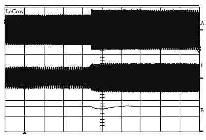
FIG. 66 DC source control behavior in case of nonlinear load transient
regime iL [10 A/div], is [10 A/div], vdc [200 V/div
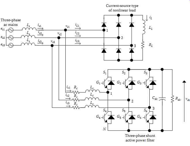
FIG. 67 System configuration.
8. Three-Phase Shunt Active Power Filter
In this section, both indirect and direct current control techniques to generate current reference for APFs are presented. These techniques are based on the instantaneous active current component id method, extracting. These control techniques are based on synchronous rotating frame transformation derived from the mains voltages. Simulation results show the performance of the control algorithms to compensate for harmonics and reactive power. FIG. 67 shows the system under study, where the SAPF is connected in parallel between the line and the nonlinear load. The SAPF consists of a full-bridge voltage-source PWM inverter, a dc-side capacitor Cdc, and three line inductors, namely, Lc. These latter are required to limit the ripple of the compensator current ic. The SAPF topology is suited for current-source type of nonlinear loads. A three-phase diode bridge rectifier feeding a series R-L circuit on its dc side represents the nonlinear load. The converter losses are represented by shunt resistance Rdc connected in parallel with the dc bus capacitor.
8.1 Current References Extraction
Generally, the control of a shunt APF is composed of two interconnected loops. The first inner loop controls the currents in order to achieve a desired filter current that is usually based on the sensed load currents, actual filter currents, supply voltages, etc. The second outer loop regulates the dc bus voltage. This voltage may vary during the transient regime depending on the control algorithm used and the losses of the inverter. The overall filter control loops should insure the following criteria:
• The generation of a suitable current reference set point that is determined from harmonic load current extraction procedure
• Sending the suitable switching signals pattern to the controllable semiconductor device's gates so that the filter current tracks its reference
• Achieve good regulation of the dc bus voltage To determine the set of the load harmonics content, the SRF harmonic method is used [19,20]. This presents the advantage of being robust against the fluctuations of supply frequency and guarantees the conservation of electrical amplitude values (currents and voltages); moreover, a phase-locked loop (PLL) allows synchronizing the SRF frequency with that of the network. Furthermore, this method possesses good qualities in term of stability and of transient (speed and quality of the response during a step of load). Finally, it directly delivers Park current references components.
8.1.1 Phase-Locked Loop Circuit
A numerical PLL ( FIG. 68) determines the phase angle θ of the source voltage, which is required for the dq transformation [19]. Therefore, the three-phase voltages vs1, vs2, and vs3 are measured and the reactive or q-component vsq of these voltages is calculated. A PI controller is used to control the angular frequency. So, if the q-component is zero the phase voltage and the angle θ are in phase.
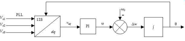
FIG. 68 Phase-locked loop.
8.1.2 T he Direct Current Control Technique of SAPF
In the direct current control technique the switching signals for SAPF devices are obtained by comparison of reference (ic1 *, ic2 *, and ic3 *) and sensed (ic1, ic2, and ic3) currents of the SAPF. This technique allows the compensation of either harmonics, reactive power, or both. This is due to the fact that the reactive energy draws a nonzero dc component (̅iq) along the q axis. The sensed three-phase load currents iL1, iL2, and iL3 in the Park reference frame are transformed into the rotating reference frame dq by using the following matrix transformation:
The active dc component ̅id represents the positive sequence at the fundamental frequency of the sensed load current. The reactive dc component ̅iq represents the positive sequence at fundamental of the reactive power. The ac components i˜d and i˜q represent the total harmonic content of the load current. These dq components are obtained at the output of a high-pass filter having id and iq as inputs. A low-pass filter with a subtracted forward action synthesizes the high-pass filter. The dc components are then eliminated, and only the ac components remains in the output signals i˜d and i˜q. The error signal between the reference value vdc * and the sensed feedback value vdc is processed through a PI controller to obtain Icm, which is added to the oscillating harmonic current ....
Note that the signal Icm is the peak value of the fundamental current Ic used to compensate APF losses. In this case, the active filter needs to compensate for the harmonics and the reactive power.
The block diagram of the synchronous rotating dq reference frame of the SAPF direct current control algorithm is shown in FIG. 69.
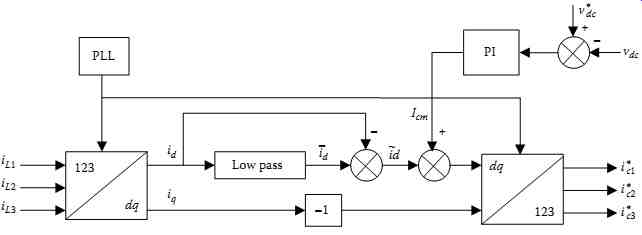
FIG. 69 Direct current control algorithm of SAPF system.
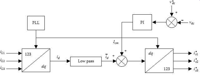
FIG. 70 Indirect current control algorithm of SAPF system.
8.1.3 T he Indirect Current Control Technique of SAPF
In the indirect current control technique, the switching signals for SAPF devices are obtained by comparison of reference (is1 *, is2 * and is3 *) and sensed (is1, is2 and is3) source currents. The d and q axes reference supply currents are expressed as follows:
8.2 Control Technique Principle
The inverter control technique uses the B-PWM principle. The control signals (βi, i = 1,2,3 and −1 < βi < 1, see FIG. 73) are compared to a triangular carrier VPWM. Each of the three legs has an independent functioning, and the switches of the same leg work in a complementary fashion. The inverter output voltage evaluated with respect to the point N takes two values, namely, vdc and zero depending on the sign of βi − VPWM. If the PWM frequency is sufficiently high, we can consider that the output mean value of the instantaneous PWM voltage over a switching period is very close to βivdc.
Moreover, if the sum β1 + β2 + β3 is zero, the following current equations hold:
8.2.1 Signal Generation for the Inverter Switches
In the direct current control, the reference currents (ic1 *, ic2 *, and ic3* ) designed from the control algorithm are compared with the sensed currents (ic1, ic2, and ic3). Then the residual signal feeds a controller having a limiter at its output. The control law provides the modulation βi considered as the direct image of the voltage mean value at the input of the inverter, which is compared with a triangular carrier resulting in the switching signal to the gate ( FIG. 71).
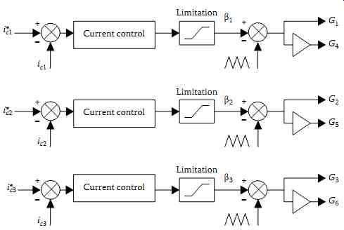
FIG. 71 PWM principle of gating signal generation for direct current
control.
In the indirect current control, the modulation βi is obtained from the filter output current regulator as shown in FIG. 72.
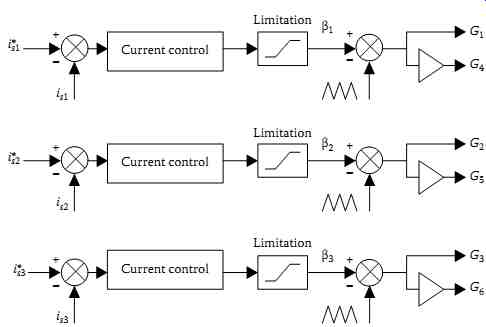
FIG. 72 PWM principle of gating signal generation for indirect current
control.
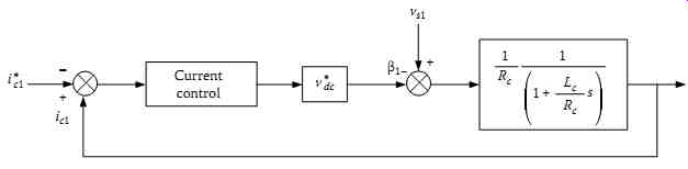
FIG. 73 Block diagram of a single-phase current control loop.
8.2.2 Current Control Loop Design
Assume that the sum β1 + β2 + β3 is zero, in other words, the current of a given phase depends only on the output regulator of the same phase. Note that this assumption is valid only in a two-loop structure, but may be considered as a big simplification in a three-loop structure, especially when the system is not perfectly balanced and is not in its steady-state regime. FIG. 73 gives a block diagram of a single-phase current control loop.
The regulator used in the different loops is of PI type. The transfer function of a typical PI regulator is given by ...
The coefficients kp and ki are chosen so that the overall closed system behaves as an optimal second order having two complex conjugate poles with a damping coefficient ξ = 0.707. They may be expressed in terms of the damping coefficient and the natural frequency ωn by Equation 38.87. For instance, the system is represented by a couple of interconnected loops. An internal fast current loop ic and an outer slow voltage vdc loop.
The PI regulator for the outer voltage loop is designed following the average model basis by considering a perfect current tracking. Whereas, the PI regulator for the inner current loop is designed independently of the outer one, in other words, the voltage vdc is assumed to be already settled. Hence, the PI regulator is synthesized regarding two transfer functions F1(s) and F2(s). The harmonic frequency range is (1 < h < 40).
With the given parameters: damping ratio ξ = 0.707, and natural frequency ωn = 50,000 rad/s, one can obtain: kp = 0.1167 and ki = 4,167, the bandwidth of the regulator should be able to respond to these criteria.
TBL. 3 System Parameters Used for Simulation
8.3 Simulation Results
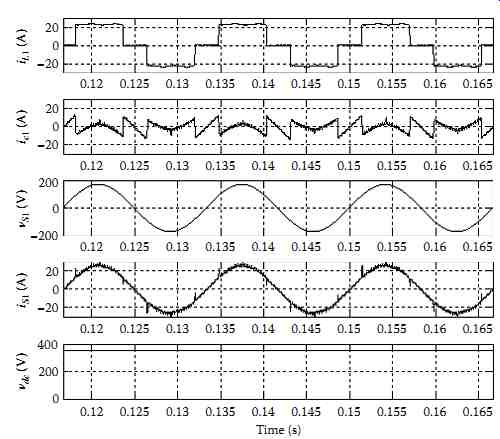
FIG. 74 Steady-state waveforms of the SAPF system with direct current
control.
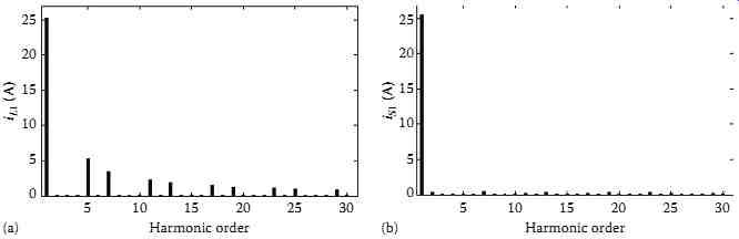
FIG. 75 Spectrum of phase 1: (a) load current and (b) source current
after compensation with the direct current control of SAPF.
In order to validate the accuracy of the direct and indirect control algorithms, the system described previously was built and simulated. The source current waveforms of the simulation results have been analyzed to obtain their THD under varying load conditions. It is simulated using the parameters as given in TBL. 3. The goal of the simulation is to present four different aspects: (a) harmonics and reactive power compensation for the direct current control technique, (b) harmonics and reactive power compensation for the indirect current control technique, (c) response of indirect current control to load variations, (d) compensation of harmonics and reactive power for indirect current control under distorted ac source.
8.3.1 Harmonics and Reactive Power Compensation for Direct Current Control
The simulation results of the system with direct current control algorithm are shown in FIG. 74, where the load current (iL1), SAPF current (ic1), supply voltage (vs1), supply current (is1), and dc bus voltage of the SAPF (vdc) are presented. The output voltage of the dc bus is stabilized at 350 volts. One can observe that the direct current control algorithm suffers from the problem of excessive switching ripples that are caused by the discontinuity abrupt in the load current that causes inadequate control response; therefore, is an instantaneous compensation of the load harmonics necessary to avoid such control loss? The harmonic spectrum of the current is measured 29.17%, whereas the compensated supply current THD is 3.68%.
A graphical representation of both load and supply currents are depicted in FIG. 75a and b.
8.3.2 Harmonics and Reactive Power Compensation for Indirect Current Control
The simulation results of the system using indirect current control algorithm are shown in FIG. 76 where the load current (iL1), SAPF current (ic1), supply voltage (vs1), supply current (is1), and dc bus voltage of the SAPF (vdc) are depicted. It is found from this figure that the supply current exhibit a ripple-free sinusoidal shape. The harmonic spectrum of the supply current is shown in FIG. 77. The THD of the source current is reduced from 29.17% before compensation to 1.94% after compensation.
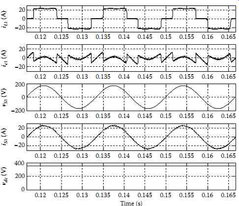
FIG. 76 Steady-state simulated waveforms of the SAPF system with the
indirect current control.
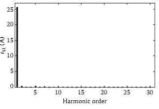
FIG. 77 Spectrum of phase 1 source current after compensation with
the indirect current control of SAPF.
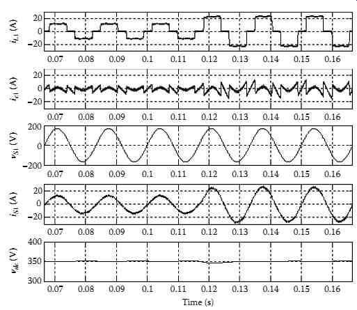
FIG. 78 Indirect current control response to load variation.
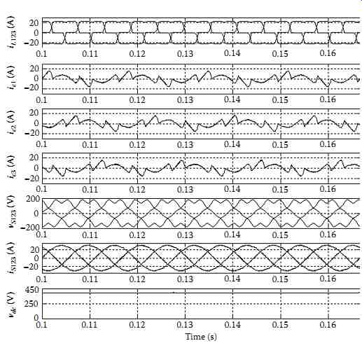
FIG. 79 Steady-state response of indirect current control under distorted
ac source.
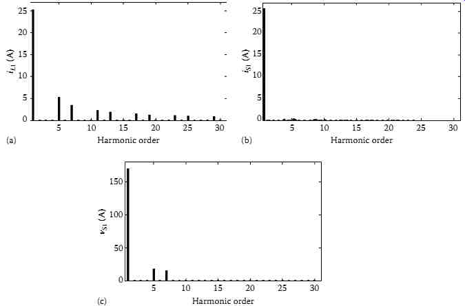
FIG. 80 Spectrum of phase 1: (a) load current, (b) source current after
compensation, (c) source voltage.
8.3.3 Response of SAPF with the Indirect Current Control Load Variation
In practice, the load power demand is usually subject to variations. Hence, it is necessary to examine the performance of the system under such disturbances. FIG. 78 shows the response of the SAPF system for a step increase of 100% of the load current at t = 116.7 ms. In other terms, the value of the load resistance is changed from 24 to 12 Ω, during which the system maintains full compensation by forcing unity PF operation without occurrence of switching ripples in the supply current. The results confirm the good performance of the compensator for a rapid change in the load current. Thus, the indirect current control algorithm offers better response.
8.3.4 Harmonics and Reactive Power Compensation for Indirect Current Control under Distorted AC Source
The purpose of the compensation is to obtain a sinusoidal current whatever the level of distortion in the source voltage. The three-phase load currents (iL123), the SAPF currents (ic123), the distorted supply voltages (vs123), the supply currents (is123), and the dc bus voltage of the SAPF during steady-state operation are shown in FIG. 79. These waveforms show the controller capability to compensate for nonlinear load currents under this severe distorted three-phase supply voltage. It is important to notice that the supply currents are kept balanced and free of harmonics. FIG. 80 illustrates the harmonic spectrum of phase 1 supply voltage, load, and supply currents. The imposed THD on the source voltage was 13.78%. The measured THD of the phase 1 source current is, therefore, reduced from 29.17% before compensation to 1.66% after compensation. These results demonstrate the robustness of the proposed controller.
9. Summary
This chapter presents the power-quality related problems and some mitigation techniques. Current power quality issues are discussed and the problems stated. The harmonics are defined and their causes and effects are explained. Various methods in use in mitigating the power quality problems are identified and presented. A large number of active filter configurations are available to compensate harmonic current, reactive power, neutral current, unbalance current, voltage sag, swell, and flicker. A study of two current control algorithms has been made and implemented on SPSAPF, in order to compensate current harmonics and reactive power generated by the nonlinear load. It has been shown that the indirect current control method offer ripples- and distortion-free supply current. Through its simplicity, it requires less hardware and offers improved performance. It is robust against abrupt changes in the load.
In addition, the bipolar and U-PWM techniques are used to generate the gate signals for the switches.
The U-PWM technique has the major advantage of eliminating the groups of harmonics that are centered on the odd multiples of the switching frequency. Furthermore, it requires a relatively reduced output filter, due to the high selected cut-off frequency that can be chosen in the neighborhood of the switching frequency. Simulation and experimental results have confirmed the superiority of the indirect current control technique performance compared to that of the direct current control technique when applied to a SPSAPF and the predicted good performance of the U-PWM controller with respect to the B-PWM controller. Two control methods for three-phase SAPF are applied to compensate harmonics, reactive power under distorted ac source has been discussed. The results of indirect current control are free from distortion in supply currents during steady-state and transient operating conditions. The indirect current control is robust against abrupt changes in the load and distorted ac source. Moreover, the later is easy to implement, and shows robustness and very good performance during both steady-state and transient operations.